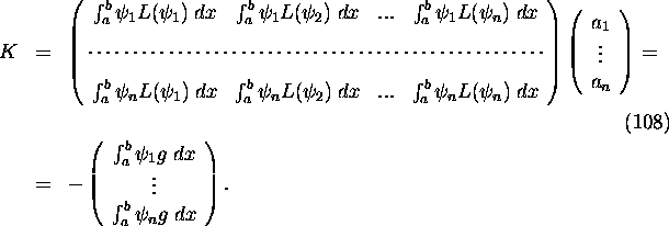
In the Galerkin's method the functions V_i(x) in (82) are defined as

Inserting (106) in (88) yields

The linear system (92) becomes

Example 1: We consider the two point boundary value problem



The function g(x) and the differential operator L are determined as

The two point boundary value problem (109)-(110) has the exact solution

Next we approximate the solution of (109)-(110) with trigonometric series

The boundary conditions (110) are satisfied if

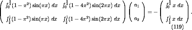
Taking n=2 in (113) we get approximation u^* with two terms as

Comparing (76) and (115) yields

Substituting and in (96) gives linear system

According to the point collocation method we choose the collocation points x₁, x₂ and solve (117) with respect a₁ and a₂. For and one obtains and

Subdomain collocation method leads to the following solution

Taking (two subdomains with equal length) we can write the system (99) as

The system (119) has solutions and therefore

Let us use the least square method now

For the present example the system (105) reduces to

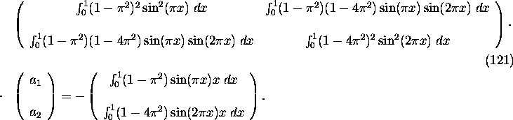
Solving (121) we get and

Galerkin's method gives the following solution

For the considered example the system (108) reduces to

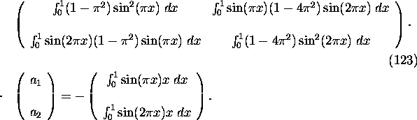
Solving system (123) yields and therefore

Comparison of solutions:

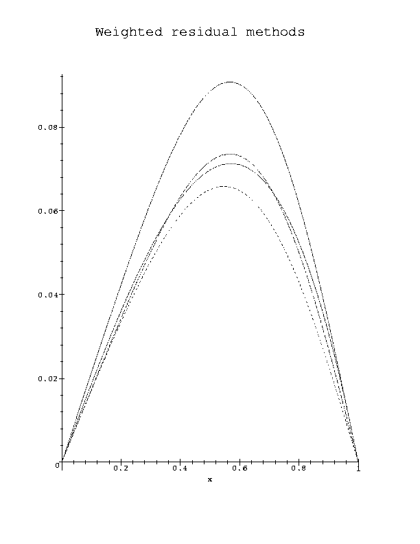
It is seen in Fig. 1., that the numerical results, obtained by four weighted residual methods are quite close to the exact solution. However, in present example only two terms in trigonometric series are considered.

Exercises

1. Solve the two point boundary value problem (109)-(110) taking n=3 and n=4. Compare results.