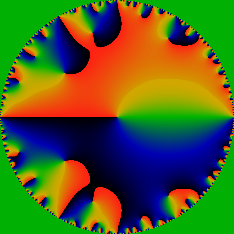
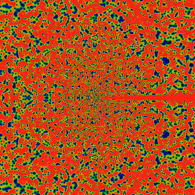
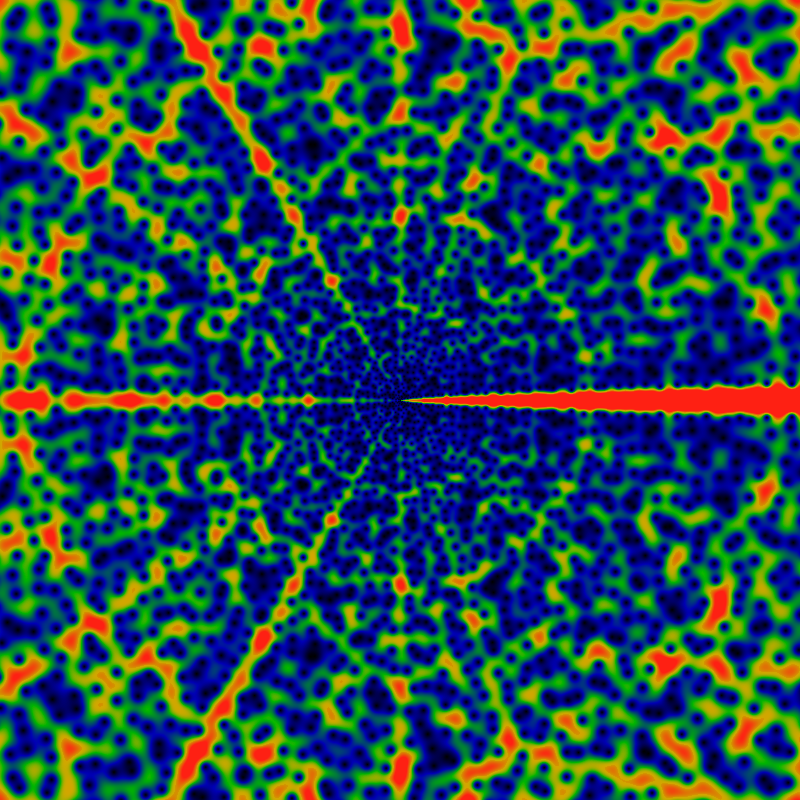
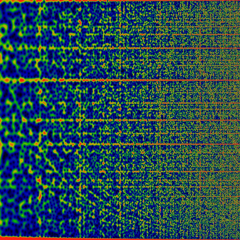
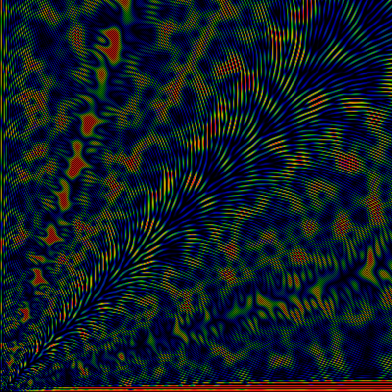
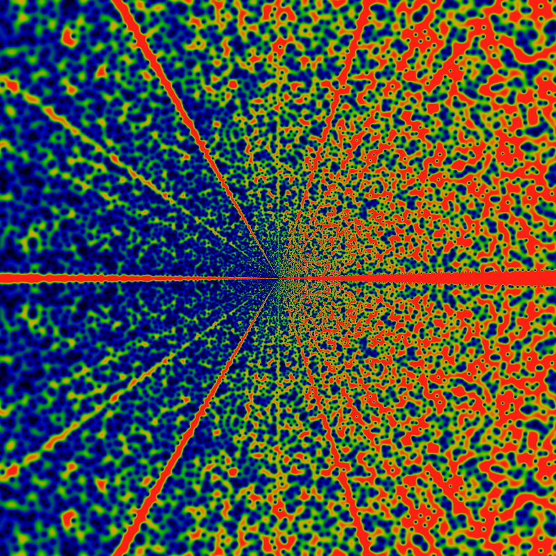
Immediately below is a phase plot of the ordinary generating function G(gpf; z) = Σn=1∞ gpf(n) zn for complex z. This function has a radius of convergence of one, with what appears to be essential singularities scattered all about the unit circle. The function is not obviously any kind of modular form, but is suggestive of some sort of theta function. That is, there is some vague fractal self-similarity-ish behavior, which is very highly typical of any sort of modular form or function (see the number theory page on this site); however, its not in any "obvious" form that e.g. the j-function or the Eisenstein functions would have. Or maybe its just another "random" hyperbolic function, as concluded on the above-mentioned number theory page. Hmmm...
By "phase plot", it is meant a visualization of the arctan of the function, which gives just the phase of the complex value of G(gpf; z). The color coding is such that red is a phase of +pi, green is a phase of zero, and black is a phase of -pi. The sharp red-black transitions are where the phase wraps around by 2pi. These lines can only terminate on zeros and on poles. Here, the lines that terminate inside the unit circle all terminate on zeros; the edge of the circle is ringed with poles (and zeros). The exterior of the unit circle is colored green: there is no analytic extension outside of the unit circle.
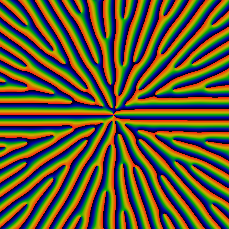
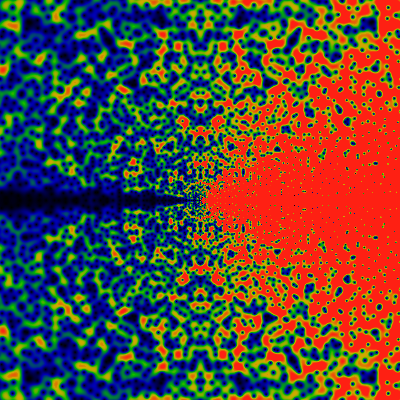
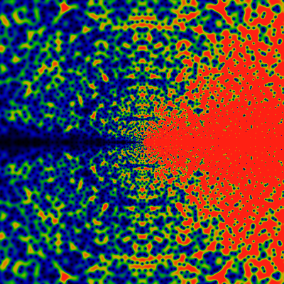
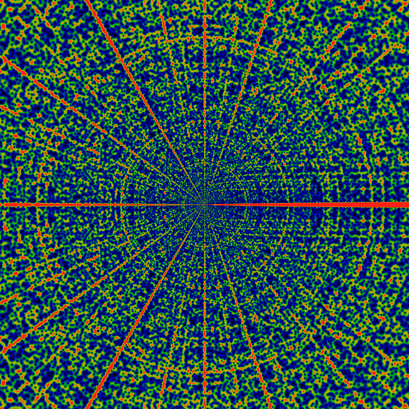
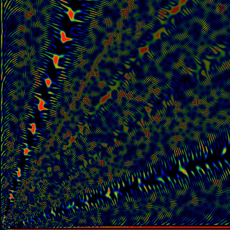
Immediately below is a phase plot of the exponential generating function EG(gpf; z) = Σn=1∞ gpf(n) zn / n! for complex z. The color scheme is the same as above.
Attention: there is a "minor" error from this point onwards: everywhere where there is a discussion of EG(gpf; z), it is actually a discussion of EG(ngpf; z) where ngpf(n) = n*gpf(n). What happened is that the numerical codes were off-by-one in computing the factorial: the numerical code accidentally computed (n-1)! instead of n! in the sum above. Amazingly (interestingly) this does not have much of an impact, as the section discussing shifts, below, indicates. However, its still annoying and so all the corrections are being made. The corrected page is here.
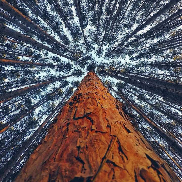
This function appears to be entire! The width of the figure is 120; that is, it graphs the domain -60 ≤ x,y ≤ +60 for z=x+iy. The rays all appear to terminate on zeros of the function; there do not appear to be any poles anywhere (except at infinity, of course). But then, this should be clear, as gpf(n) is bounded by n.
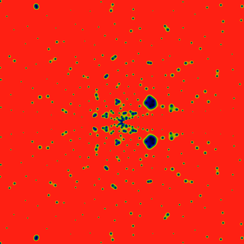
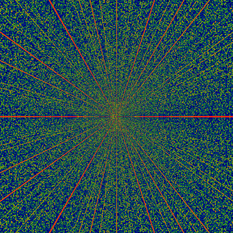
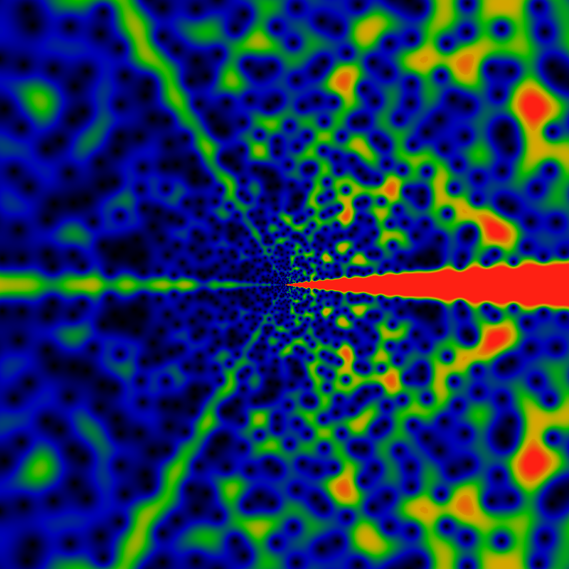
Below is the absolute value of the exponential generating function, explicitly showing the location of the zeros as black dots. Note that EG(gpf; z) diverges as exp(|z|) for large |z|; thus the color scale below actually displays EG(gpf; z) exp(-|z|) / |z| to make the zeros more easily visible. The color map is such that red corresponds to values of 1.0 or greater, and green to values around 0.5.
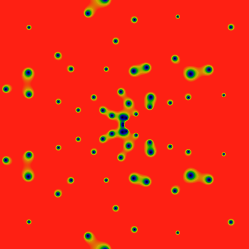
The zeros, again, but with the color maps scaled by 0.24.
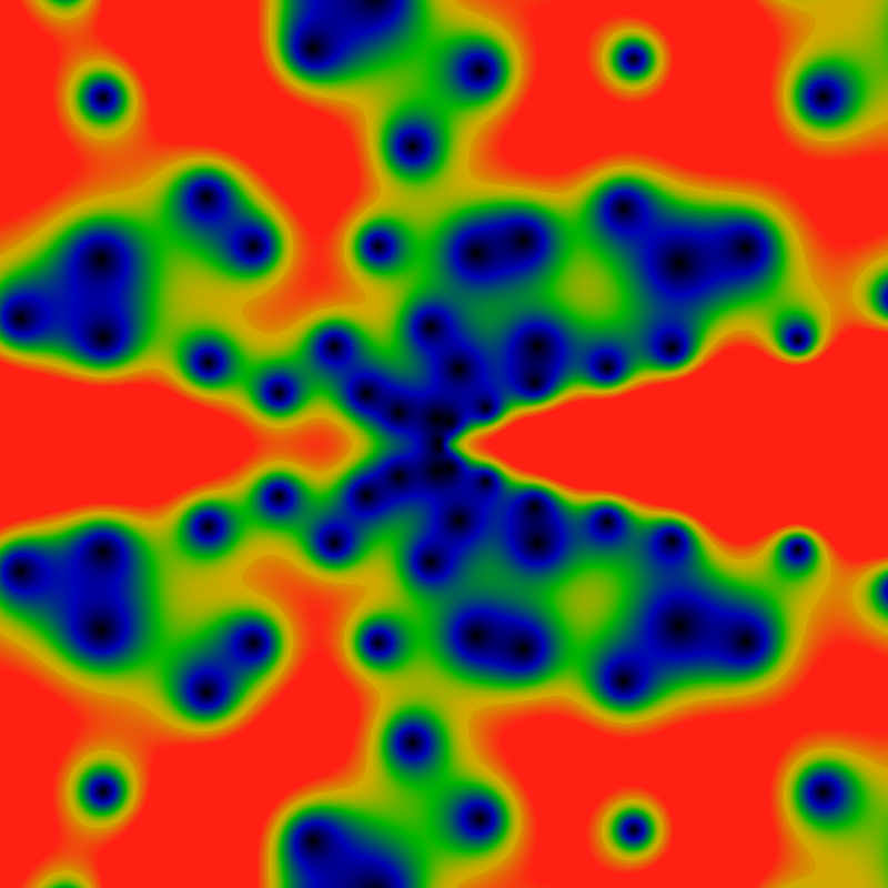
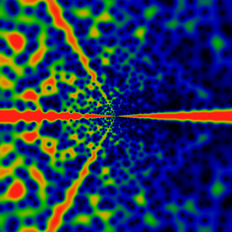
The zeros, again, but with the domain (x,y) ranging from -360 to +360. The big blue-black blobs to the right are five different zeros fairly close to each other.
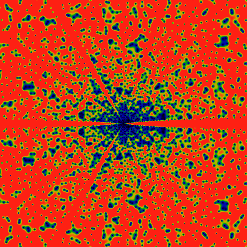
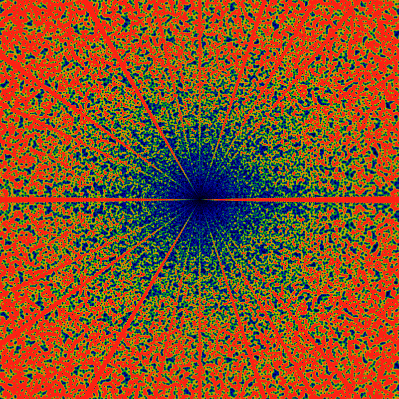
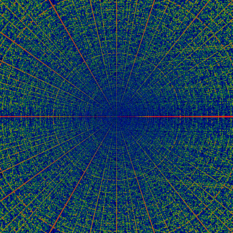
And again, but with the domain (x,y) ranging from -2160 to +2160. The colors are scaled to make the large-|z| zeros more clearly visible. This has the side-effect of highlighting rays, lanes which are free of any zeros. Rays for the cyclic groups Z2 and Z3 are clearly visible, and with some peering, the rays for Z5 can be seen as well. There's a hint of Z7. Notably absent are rays for Z4. This seems to lead to a natural conjecture that zeros never occur on a ray for Zp, p prime.
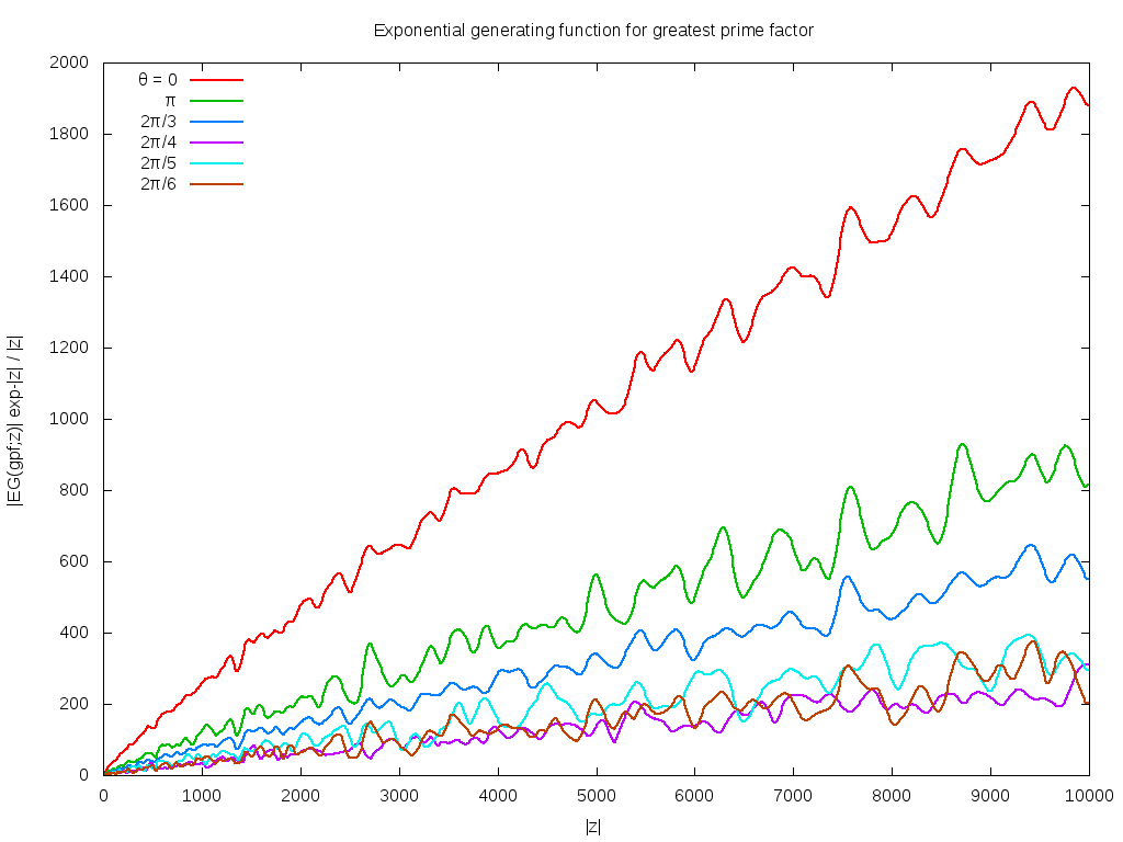
The above conjecture can be explored by taking slices along rays, shown below. It shows six slices, taken along the direction z=|z|exp iθ for θ=0, π, 2π/3, 2π/4, 2π/5, 2π/6 The leading divergence of |z|exp|z| has been removed, leaving a divergence that seems to be about of order |z|/log|z|. Notable in this graph is that no zeros are visible along the rays for θ=2π/4 and θ=2π/6. This suggests the the above conjecture is in fact, incorrect.
Most notable about this picture is the pronounced smooth oscillations along each ray. It's visually clear that the wavelengths get longer as |z| gets larger. Closer examination shows that the wavelength goes as the square-root of |z|.
A similar exploration of rays directed along quadratic irrationals suggests that such rays pass very close to zeros on a number of occasions, but none actually pass through a zero. The below shows a phase plot of one such ray, graphing the real vs imaginary part of EG(gpf; z) for |z| running from 0 to 1000. The close passes are visible: recall that since the leading exponential scaling is removed, the close passes visualized here are indeed very close.
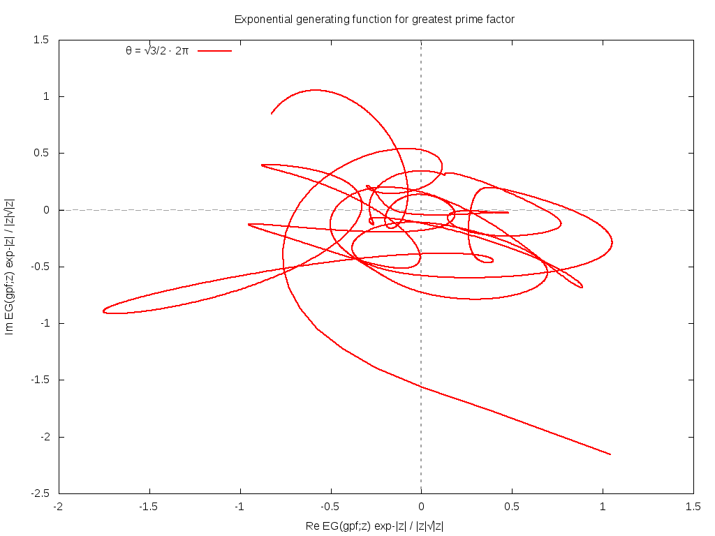
So where are the zeros located? Hard to say. The exploration of other angles, including simple fractions (without any factors of pi) suggests that these, too, manage to not hit any zeros, at least, not for |z| < 1000, although the ray for θ=1/3 really sure does come very, very close.
Here's a table of the 11 zeros nearest the origin. The coding is such that z=r exp(i π φ) = x + i y. Accuracy is good to about the last digit. Plouffe's inverter doesn't seem to know any of these numbers. They're presumably all some unknown transcendentals.
| r | φ | x | y |
|---|---|---|---|
| 0.88022349562601 | 0.83295289206477 | -0.76176934606451 | 0.44102252283587 |
| 3.2375048946125 | 0.42458721923649 | 0.75986223121855 | 3.1470696420968 |
| 3.7441361185659 | 0.59817818048564 | -1.136602428757 | 3.5674486952574 |
| 7.4736771339129 | 0.23110162504623 | 5.5889493606786 | 4.9618035980621 |
| 7.511312297442 | 0.80582634942347 | -6.1565697810839 | 4.3030757558226 |
| 10.41426766772 | 0.44047959714246 | 1.9360237252942 | 10.232730974183 |
| 12.602613307375 | 0.81645934805374 | -10.564968103744 | 6.8707576832617 |
| 14.800600506967 | 0.19203401986558 | 12.187879585189 | 8.39722374263 |
| 15.997814072863 | 0.53774902696863 | -1.8927698515501 | 15.885448605531 |
| 18.340908478517 | 0.25911033247266 | 12.592535370681 | 13.334803213977 |
| 19.957065054996 | 0.768238424116 | -14.896747647415 | 13.280487759815 |
Before one gets too excited, its worth asking: how much of the general shape of this function is due to the fact that the greatest-prime-factor series is being used, and how much is "generic", shared by any similar series? To answer this question, one can generate random series rs(n) that roughly resemble gpf(n), for example, having the property that 2 ≤ rs(n) ≤ n, but otherwise having a uniform distribution in this range. In such a case, one finds that EG(rs, z) does have zeros scattered all over the complex plane, in a roughly similar distribution; however, the rays are completely absent, as can be seen below.
Perhaps the rays are due to the primes? One can consider a random distribution rps(n) having the property that 2 ≤ rps(n) ≤ n and also that rps(n) is prime. Below are EG(rps, z) for two such random sequences. No rays, but hints of rings! Curious! And also, an odd left-right symmetry! Clearly, more work can be done in this general area.
Anyway, some more views of EG(gpf, z). This one for the domain -20000 ≤ x,y ≤ +20000 for z=x+iy. This time, a ray at Z4 is visible. The width of the rays does not follow any obvious hand-waving pattern.
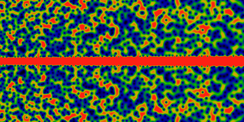
Some trees in a forest... photo by MIAN FAISAL.
The below is for the domain -125000 ≤ x,y ≤ +125000 for z=x+iy. It uses a different normalization than the earlier pictures: it multiplies GE(gpf;z) by a term 0.4 r-2log2(r) exp(-r) where r=|z|. That is, the leading exponential divergence is easily brought under control by the exponential term, leaving a much weaker divergence. dividing by r2 seems to over-compensate; multiplying by the squared log term seems to be just about right. The factor of 0.4 is just what is needed to get a pleasing color balance in this picture: again red areas represent values greater than 1, green are the values near 0.5, and blue-black are areas of about 0.2 or less. (No other processing is applied to this image, nor to any other image on this entire website).
The most notable aspect of this image is the narrowing of the rays. If one asked for the number of zeros in a pie-sliced wedge, and graphed that as a function of the angle, one would see a devil's-staircase type function. But, as this image shows, the treads on those stairs decrease in size as the radius of the circle increases. The rate is unclear; perhaps it goes as the square-root of the radius? That is, there are lanes that are completely free of zeros; these lanes get wider for larger radius, but at a sub-linear rate. They would have to, to make room for finite-width lanes for every rational!
The widening of these zero-free lanes is one of the more interesting aspects of this image. Clearly, there is a suggestion of a ray for every rational. The simplest rationals have the widest lanes; but what, exactly, constitutes "simplest", here? If the rays are arranged according to widths, do they come in Farey-fraction order?
Also notable is a vague hint or suggestion of Moire patterning along the x-axis. Recall that Moire patterns occur when one regular (cyclic) grid pattern is superimposed on another, but shifted over. In this case, one regular pattern are the square pixels of the image; the other is the location of the zeros. The appearance of a Moire pattern is then strong evidence that the location of the zeros are not "random", but are correlated in some regular, cyclic way (as one moves from ray to ray). But of course it is: up above is a graph of six slices taken along a constant angle (six rays). These each show a characteristic oscillation with some very strong Fourier components. The Moire patterns are these same Fourier components, interfering with the characteristic pixel size.
How real or illusory is the Moire patterning? Below shows a close-up, running along the domain 24000 < x < 48000 and -12000 < y < 12000. Again, there is a hint of yet more structure -- diagonal arrowhead/feather lines. Individual zeros are clearly distinguishable, and it is interesting how they line up so regularly, maintaining a uniform lane.
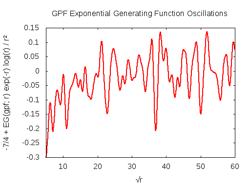
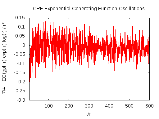
The asymptotic behavior of the generating function can be guessed at by numerical means. The graphs below show the re-scaled quantity -7/4 + EG(gpf; r) exp(-r) log(r) / r² as a function of √r. The strong periodic oscillations are clearly visible. The rescaling hides just how small these oscillations are: So, for √r = 60, one has r = 3600 and r² exp(r)/log(r) ~ 1029, and so the amplitude of the oscillations is 30 orders of magnitude smaller than the function itself! That this does indeed seem to be the correct asymptotic scaling is reinforced by the graph that shows the same oscillations out to √r = 600. This corresponds to r = 360K and r² exp(r)/log(r) ~ 2 · 10265, which is truly huge! That the oscillations are happening around 7/4 = 1.75 is just a suggestion from the graph: closer numerical work suggests that the centerline is perhaps at 1.744.
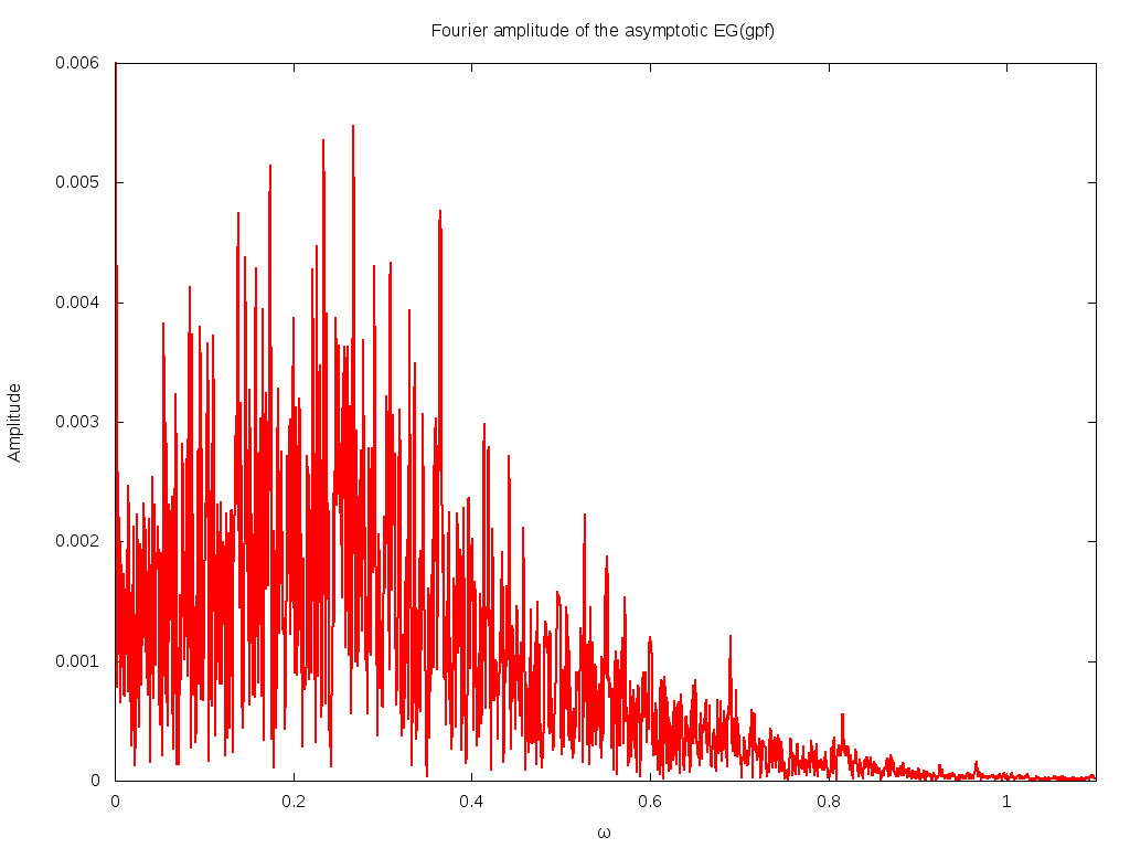
What's the Fourier spectrum? Low-frequency noise, it seems. The figure
below shows the amplitude of the Fourier components, as a function of
frequency. Specifically, this shows the amplitude √(a²(ω)+b²(ω))
where the Fourier components are
a(ω) = ∫ f(t²) cos(2π ωt) dt
b(ω) = ∫ f(t²) sin(2π ωt) dt
and where f(r) is the asymptotically rescaled generating function:
f(r) = -7/4 + EG(gpf; r) exp(-r) log(r) / r²
The integration is taken over the range 10 < t < 610.
This corresponds to the second graph above. Again, its hard to
overemphasize how small these oscillations are: the integral is
performed over a region where the generating function blows up by
265 orders of magnitude! Take some caution, however, in interpreting
the graph scale: the amplitude at any given frequency is probably either
zero or infinite; this graph is just an approximation to the true
Fourier spectrum, which presumably consists of Dirac delta functions
of various weights at various irrationals.
Perhaps the most notable feature of this graph is that, indeed, it looks very noisy: there is no obvious self-similar structure in it. Its hard to make out what the fall-off in frequency is: its perhaps cubic. In case you are wondering: no, this is NOT numeric noise; this can be most easily seen in the left figure above, where the oscillations are small and smooth; it is the Fourier components of this smooth graph that are not smooth. The calculations are performed with the Algorithmic 'n Analytic Number Theory multi-precision library (based on gnuMP); the results are verified by repeating the calculations at various different precisions.
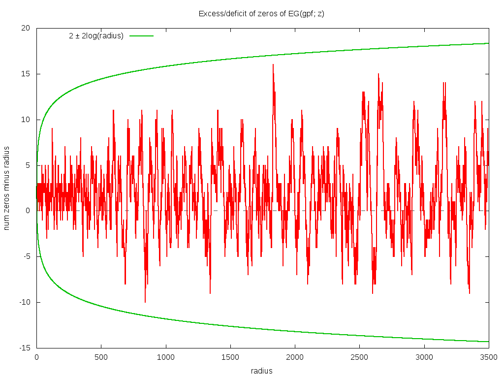
The zeros seem to be scattered very uniformly around the complex plane. How many are there? They are easy to count using Cauchy's argument principle: one performs an integral of the phase around a circle of radius r; this counts the number of zeros inside the circle. This counting is easy to perform numerically. The result is that there are almost exactly N zeros within radius N of the origin, the count being off by no more O(log(r)). The numerical work suggests that the strict bound is 2 ± log(r2) with equality holding at r=1 (there are three zeros inside of r=1, which is two more than expected). The surplus or deficit of zeros, as a function of the enclosing radius, is shown below. Note that this linear dependence on the radius means that the density of zeros is decreasing as the square root -- the area of a circle goes as r2.
Movie time! This surprised me, but what do I know? Consider the n'th derivative, with respect to z, of EG(gpf; z). Because derivatives of the exponential series yield the series itself, this derivative has teh effect of acting as a shift operator on gpf. That is, define the shift operator S acting on an arithmetic series f as (Sf)(n)=f(n+1). It follows that dnEG(gpf; z)/dzn = EG(Sngpf; z). Where might the zeroes of this function lie? Surprise! The animation below shows what happens: each frame is a shift from the prior frame. Clearly, the zeros shift towards the origin; but the overall structure is preserved. Its hard to tell, but it seems that a pair of zeros disappear each frame. Although it seems, at first, that the zeros approach the origin uniformly, it quickly becomes clear that there is some tidal shearing. Careful observation will show that sometimes, one zero races past another one.
There's another interesting thing: towards the end of the movie, on the negative x-axis, a pair of mirrored zeros coalesce into one (double) zero on the x-axis, and then split apart into two, in sequential order, one falling in before the other. Something similar also seems to happen on the ray 2π/5, although it is not clear if the two zeros actually coalesce before dropping in, or if they merely get close. At any rate, they start out roughly equidistant from the origin, but then fall in at sharply different times.
I've never explored the action of shifts on exponential generating functions before; this behavior of radial inflow is a complete suprise to me. It turns out to not be unique to gpf; the exponential generating function of shifts of any of the random series discussed above also exhibit this kind of flow. Its presumably a well-known property of the exponential generating function; its just news to me.
The movie is 108 frames long, starting from a shift of zero. The domain is -100 < x,y < +100, and so almost every zero initially visible at the start of the movie has fallen into the origin by the end of the movie.
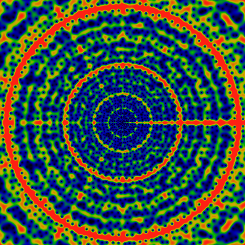
One last image. This one is for the reciprocal of the GPF. To be precise, its for the absolute value of 0.5 EG(1/gpf; z) exp(-|z|)/log|z|, with the domain (x,y) ranging from -2160 to +2160, and the color scale such that 1.0 or greater is red, 0.5 is green and blue/black is 0.25 or less. (This is the same color scale as all the other images; however, some of the other images are scaled by an arbitrary constant to make them pretty; this one is not scaled at all, but is straight as written). The image suggests (of course) that the asymptotic scaling is |EG(1/gpf; z)| ~ O(exp|z| log|z|) or thereabouts.
Clearly, there's a new feature visible here: rings! Concentric rings! Hard to tell, but, pulling out a ruler and eyeballing them, they seem to be located at powers of two: the outermost at a radius of 2048, then three more clearly visible at 1024, 512 and 256. Hard to tell, but there is a vague hint of another ring at 1536=3*512. And maybe yet many more rings! Wow! Who knew?
I lied. That's not the last image -- it pays off to keep making more. The below is the same as above, but over a domain ranging from -20K to +20K. Actually, its slightly different: it shows 24.0 EG(1/gpf; z) exp(-|z|)/ log3|z|, suggesting the asymptotic |EG(1/gpf; z)| ~ O(exp|z| log3|z|) or thereabouts. The estimate of the logarithmic terms in the asymptotic behavior is a bit ambiguous.
Newly visible are lines paralleling the positive x-axis, seeming maybe to curl around the origin in some vaguely parabolic way. There's a particularly large pseudo-parabolic orbit visible, coming in from the right, about 3/4th's of the way up, turning around the origin, and exiting abut 3/4th's of the way down (on the right, of course -- its easy to see, once you see it.)
As before, there are hints of Moire patterning along the x-axis, although this time, the scale of the picture is such that the individual zeros can still be distinctly mad out. Therefore, the Moire patterns cannot be optical pixel-scale effects -- that is, its not an effect due to the finite size of the pixels -- it does not meet the criteria for the classical, canonical definition of the Moire effect in a computer graphics image. Instead, the Moire patterning seems to actually exist within the function itself! This suggests that perhaps the function itself can be decomposed as a sum of "layers", each layer consisting of a very regular oscillatory pattern, with only the sum of the patterns resulting in the apparent chaos of the image.
What are all these features? How are they to be described? What do they correspond to? One can't help but get the sense that this is the projection of some structure on some bundle, some structure built of sheafs and germs, but quite how to get that is unclear.
Below is same as above, except for a domain of -120K (= -1.2e5) to +120K (and a slightly bluer color scale). Note the extremely vague and hard to see hints of parabolic orbits facing to the left (not just the right!) There are also hints of other traceries, but its hard to say if these are merely optical, visual field effects or if they have some basis in mathematical reality.
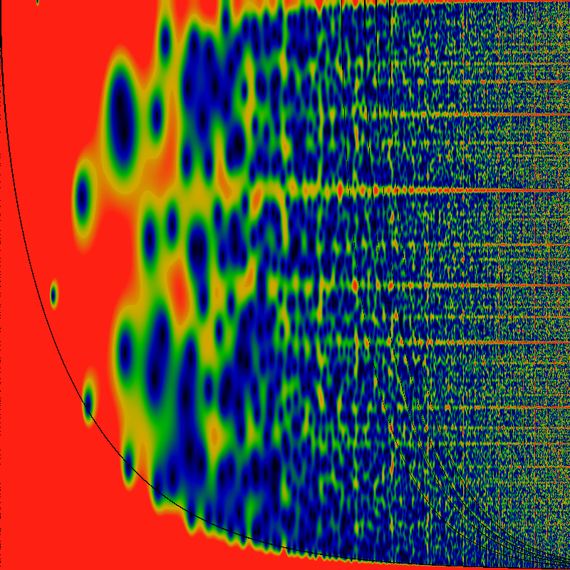
What are these parabolic-like orbits? Well, there's an alternate plot that makes curve-fitting easier. The below unwinds the the graph from around the origin, showing instead, as the above, 24.0 EG(1/gpf; z) exp(-|z|)/ log3|z|, except that here, z=r exp(iθ) with θ running along the vertical axis, from 0 to π. Along the horizontal axis, r is plotted on a logarithmic scale, so that r runs from 1 on the left to 65536 on the right. Superimposed on this figure are five hand-fitted black lines. One tries to capture the edge of the root-free zone. This line is given by sin θ/2 = 1/√r. Note the radical. Careful examination shows that at least a few zeros appear on the wrong side of this line -- the shape seems to be only approximate. Four more lines try to fit the pseudo-parabolas. The fits are OK on the large-r asymptotic region, but poor in the small-r region. The four that are drawn are given by
| 768/r = sin θ/2 |
| 1200/r = sin θ/2 |
| 1500/r = sin θ/2 |
| 1948/r = sin θ/2 |
| 7200/r = sin θ/2 (not drawn) |
That happend to the circles? They should be vertical lines in the above! Well, they are still there, just too narrow to be visible in the above. They do become visible, below: five evenly spaced vertical lines, using the same mapping and logarithmic scaling as above. The domain of r is from 1024 on the left to 65536 on the right, so the five vertical lines correspond to r=2048, 4096, 8192, 16384, and 32768, respectively. Otherwise, there is nothing particularly new in this image; everything visible here is visible in earlier images.
Just how thin are these vertical lines? The image below is a closup of the image above: in this case, r runs from (32768-650) to (32768+650). Eye-balling the red strip, it seems maybe 350 units wide -- so maybe a width of √32768=362 is a decent wild guess. Is this vertical stripe really zero-free? Hard to tell from this picture. There are lots of blue smears -- there are about 1300 zeros in this image (as shown above, there are about r zeros inside a circle of radius r). Fiddling with the color-map helps isolate some of these a bit more clearly, and it seems like there might be dozen or two zeros actually within the red stripe, rather than all the blue being just a smear from outside the stripe.
Below is 0.3 EG(1/gpf2; z) exp(-|z|), with the domain (x,y) between -2160 and +2160. The circular rings become sharply visible. The primary sequence seems to be located at powers of 2; so that, here, the outermost ring appears to be of radius 2048; the middle one presumably with a radius of 1024, etc. The other rings are presumably at other prime powers.
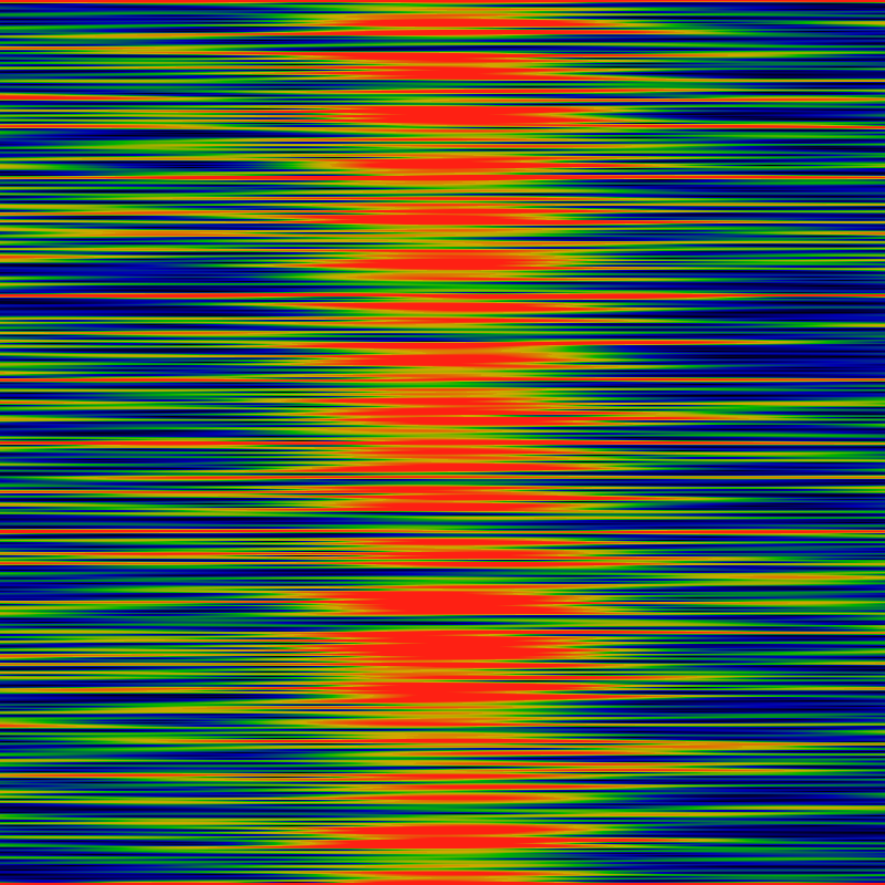
Below is an actual moire pattern! It shows the real part of EG(gpf; z) exp(-|z|). As noted at the very begining, in the phase portrait, the phase forms radially oriented fingers. Likewise, the real part of the function consists of radially oriented, roughly sinusoidal ridges and valleys. At the scale of this image, the distance between peak and trough is less than one pixel, and so by using a sharp sampling, one necessarily gets a sampling aliasing effect. The original image here is 400x400 pixels, and it shows a region 0 < x,y < 2000 (the upper-right quadrant). The moire patterning gives a hint about how the radial fingers differ from being perfectly radial.
As above, but for the region 0 < x,y < 4000. Should not be any need to point out that Moire patterning is very sensitive to the sampling frequency.
As above, but for the region 0 < x,y < 8000.
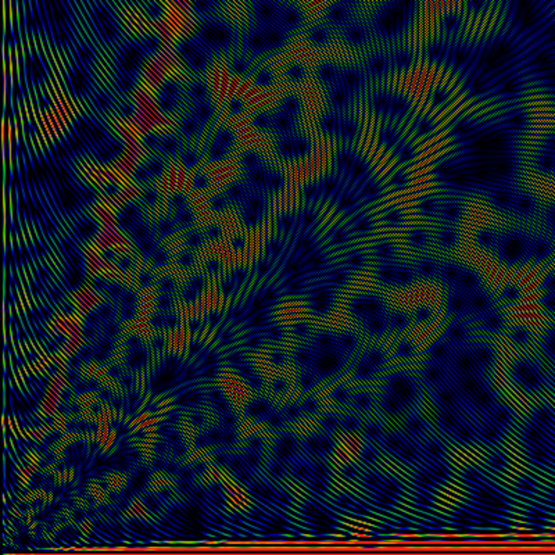
Perhaps you are starting to get bored, so I will try to wrap it up. Below is one for the rising Pochhammer symbol. Its normalized by a factorial, for convergence, so really its a binomial coefficient. Specifically, define RPG(f; z) = Σn=1∞ f(n) (z)n / (n!)2 where (z)n = z(z+1)(z+2)...(z+n-1) is the rising Pochhammer symbol. The two factorials in the denominator guaranatee convergence, as otherwise the sum is badly behaved. The color coding is as before: black is zero, green is about 0.5 and red is any value that is 1.0 or larger. The leading divergence is removed: the graph shows this: RPG(gpf,z) exp(-2 √ |z|) / |z| Notice the √ |z| in the normalization: such binomial-coefficient sums (Newton series, actually) are "well-known" to diverge in this kind of square-root fashion. (This is explored in detail in a paper by Philippe Flajolet and myself on Newton series for the Riemann zeta). Anyway -- notice again that ther seem to be zero-free rays at angles theta=0 and π of course, and at 2π/3 and, harder to discern, at 2π/5. Presumably all the other rationals are there too; they are not very clear in this picture. The domain in this picture is just huge: -1.0e6 < x,y < 1.0e6 -- this is far far wider than any of the previous images: the zeros are much, much farther apart.
One may also consider a very similar sum, using the falling Pochhammer symbol, instead of the rising one. This symbol is given by (z)n = z(z-1)(z-2)...(z-n+1). The resulting image appears below, it is of FPG(gpf,z) exp(-2 √ |z|) / |z| with normalization exactly as given and coloration as always.
Some of the first few zeros for the rising Pochhammer generating function are shown below. Note that the first two lie precisely on the real axis. The others do not seem to occur at any low rational angle (the column φ shows the angle in units of pi, thus a value of φ of one indicates the negative x-axis), although the next few seem to try to get close to the 3rd roots of unity, and the one after that the 6th root of unity. After that, there is no clear progression. As before, they are presumably transcendental, rather than, for example, quadratic irrationals, or some such.
| r | φ | x | y |
|---|---|---|---|
| 1.3949092398684 | 1 | -1.3949092398684 | 0 |
| 4.5626759564288 | 1 | -4.5626759564288 | 0 |
| 10.245898379007 | 0.64420879547681 | -4.4846874842696 | 9.2122750589292 |
| 24.83352515618 | 0.63379620727208 | -10.133683877231 | 22.671842068058 |
| 55.576607747775 | 0.3205855915997 | 29.693058011758 | 46.979587425396 |
| 72.25879634152 | 0.8121672651601 | -60.038996469216 | 40.207618080342 |
| 117.75420722502 | 0.46759200907347 | 11.968172804434 | 117.1444243612 |
| 192.15199916793 | 0.81693429156798 | -161.24015864602 | 104.51795072638 |
| 201.03591391007 | 0.25107689390384 | 141.67211584758 | 142.63397306717 |
| 285.6352301736 | 0.54737231184267 | -42.35277394865 | 282.47783498034 |
| 364.85530526812 | 0.27307016022456 | 238.63224457153 | 275.99645945745 |
| 442.19734166307 | 0.78730029361836 | -347.09323384104 | 273.97951747467 |
| r | φ | x | y |
|---|---|---|---|
| 0.72183600549901 | 0.49137876622082 | 0.019548108331473 | 0.72157126487647 |
| 10.360150450484 | 0.45106261529342 | 1.5865160932827 | 10.237953117808 |
| 23.302941560009 | 0.47588077521583 | 1.7640394756877 | 23.236076477697 |
| 57.987569085342 | 0.7605584350114 | -42.340693875438 | 39.621002139948 |
| 67.48077369795 | 0.26157732931857 | 45.949442919987 | 49.419667281528 |
| 122.32995335662 | 0.40689342952179 | 35.273809336995 | 117.13400814063 |
| 168.26853286447 | 0.78918215559082 | -132.69280305254 | 103.4742439954 |
| 224.60980862841 | 0.22477866727782 | 170.89602763141 | 145.75360672003 |
| 281.86194385292 | 0.50767619198356 | -6.7965739748906 | 281.77998859881 |
| 393.67913951173 | 0.2492135681373 | 279.06010117129 | 277.68457793146 |
| 410.84081343407 | 0.76652914265676 | -305.19542443344 | 275.03804625552 |
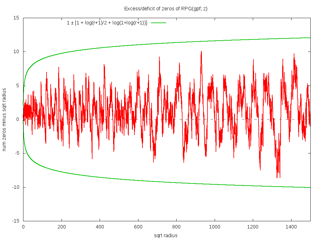
How many zeros are there? As before, we have the curious similarity: the bound on the rate of divergence of the function gives the count of the zeros. Thus, asmptotically RPG(gpf; z) seems to go roughly as O(|z| exp (2 sqrt|z|). The number of zeros inside a circle of radius |z| appears to be given by 1 + √ |z| and the error of this approximation is bounded by ± [1+log(1+|z|)/2+log(1+log(1+|z|))], as the graph below shows. This bound appears to be tight; nothing tighter seems to work. Note that this bound extends all the way to |z|=0 -- that is, it is not violated at small |z|.
Initial version: April 2016. Revised version: October 2016

Greatest Prime Factor
by Linas Vepstas is licensed under a Creative Commons
Attribution-ShareAlike 4.0 International License.