Almost all of the content here is also available as a PDF file; only the movie is missing.
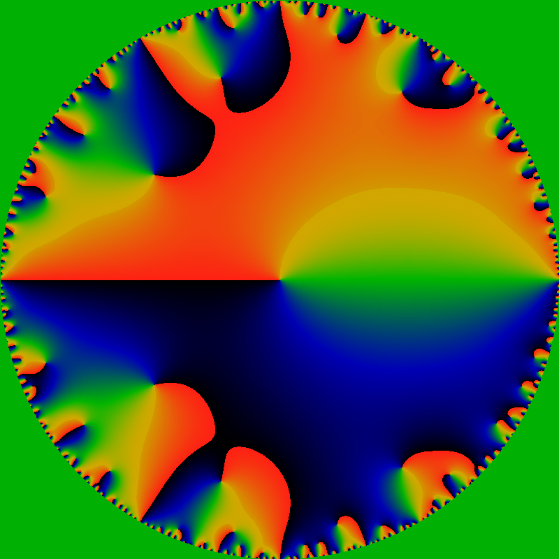
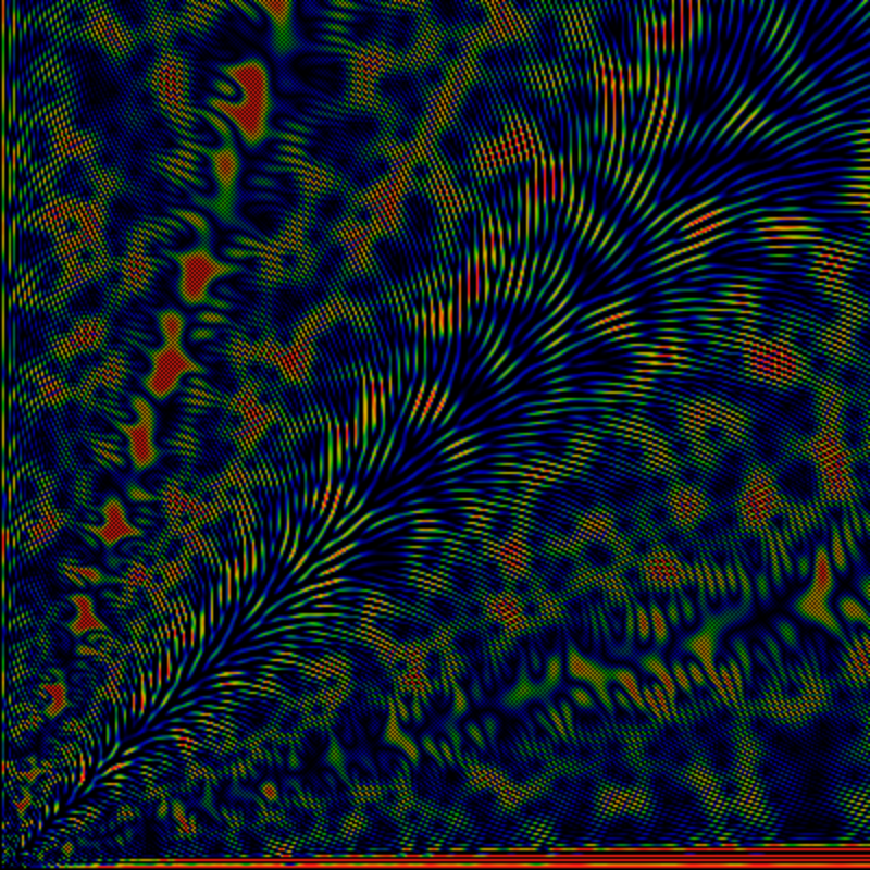
By "phase plot", it is meant a visualization of the arctan of the function, which gives just the phase of the complex value of OG(gpf; z). The color coding is such that red is a phase of +pi, green is a phase of zero, and black is a phase of -pi. The sharp red-black transitions are where the phase wraps around by 2pi. These lines can only terminate on zeros and on poles. Here, the lines that terminate inside the unit circle all terminate on zeros; the edge of the circle is ringed with poles (and zeros). The exterior of the unit circle is colored green: there is no analytic extension outside of the unit circle.
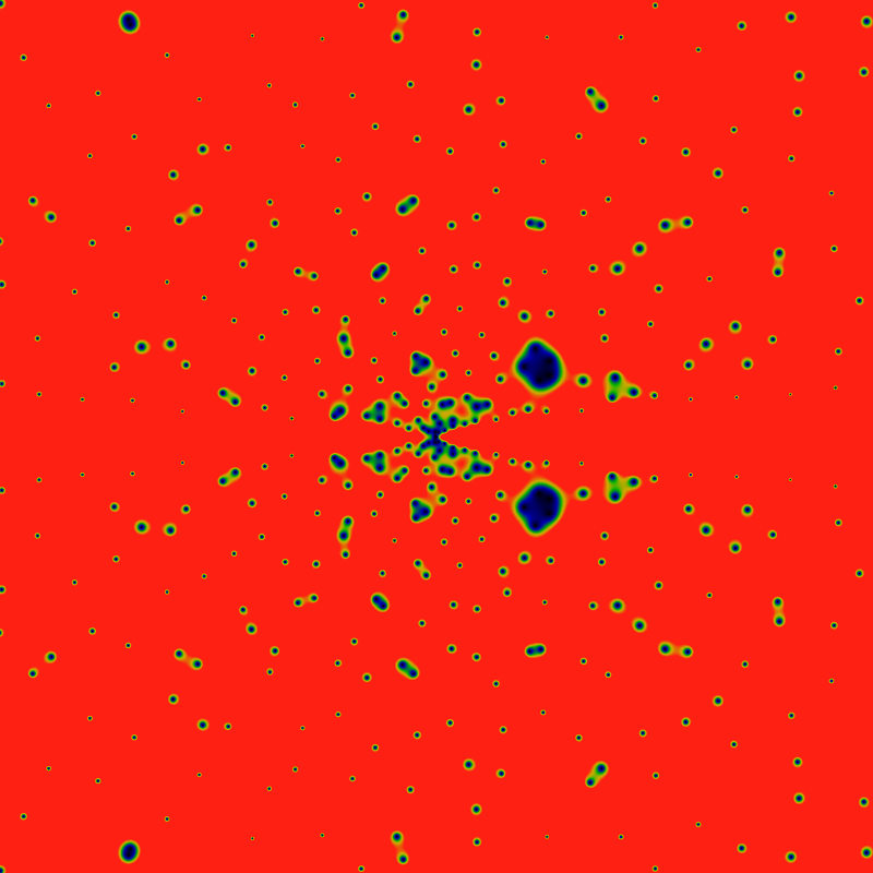
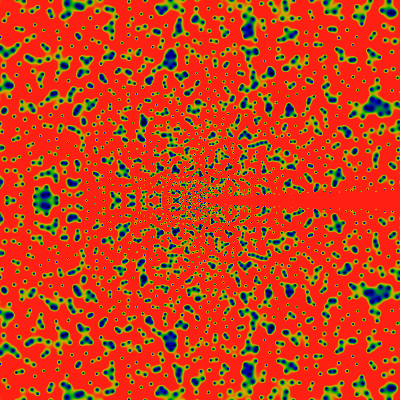
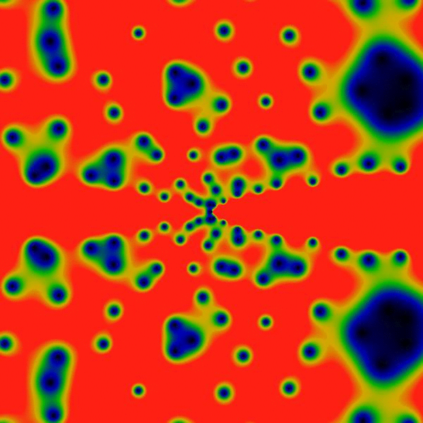
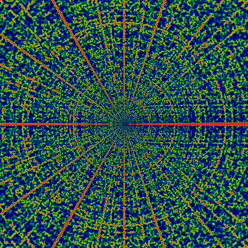
Immediately below is a phase plot of the exponential generating function EG(gpf; z) = Σn=1∞ gpf(n) zn / n! for complex z. The color scheme is the same as above.
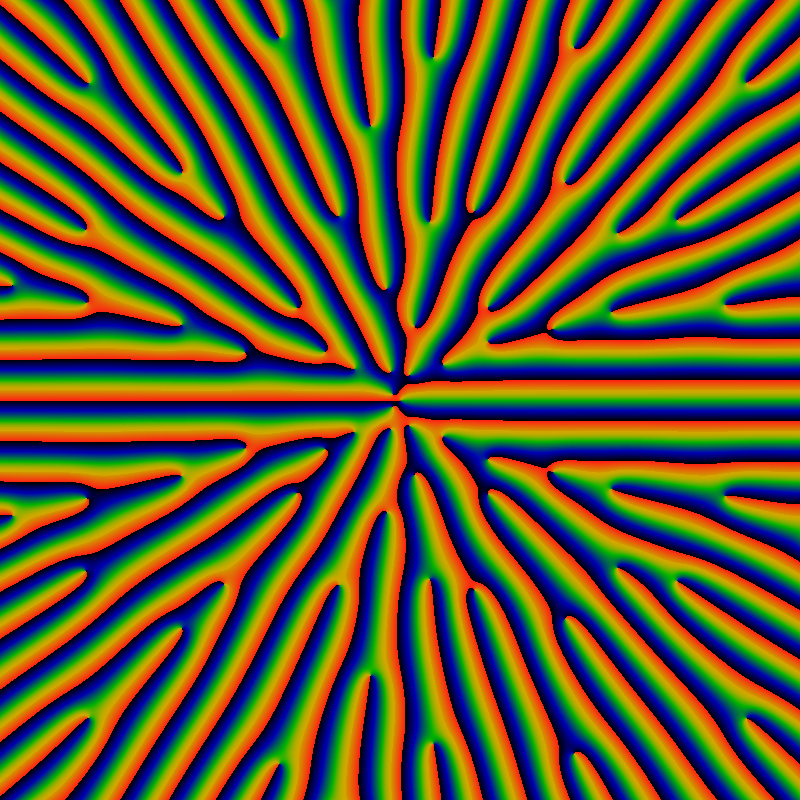
This function appears to be entire! The width of the figure is 120; that is, it graphs the domain -60 ≤ x,y ≤ +60 for z=x+iy. The rays all appear to terminate on zeros of the function; there do not appear to be any poles anywhere (except at infinity, of course). But then, this should be clear, as gpf(n) is bounded by n.
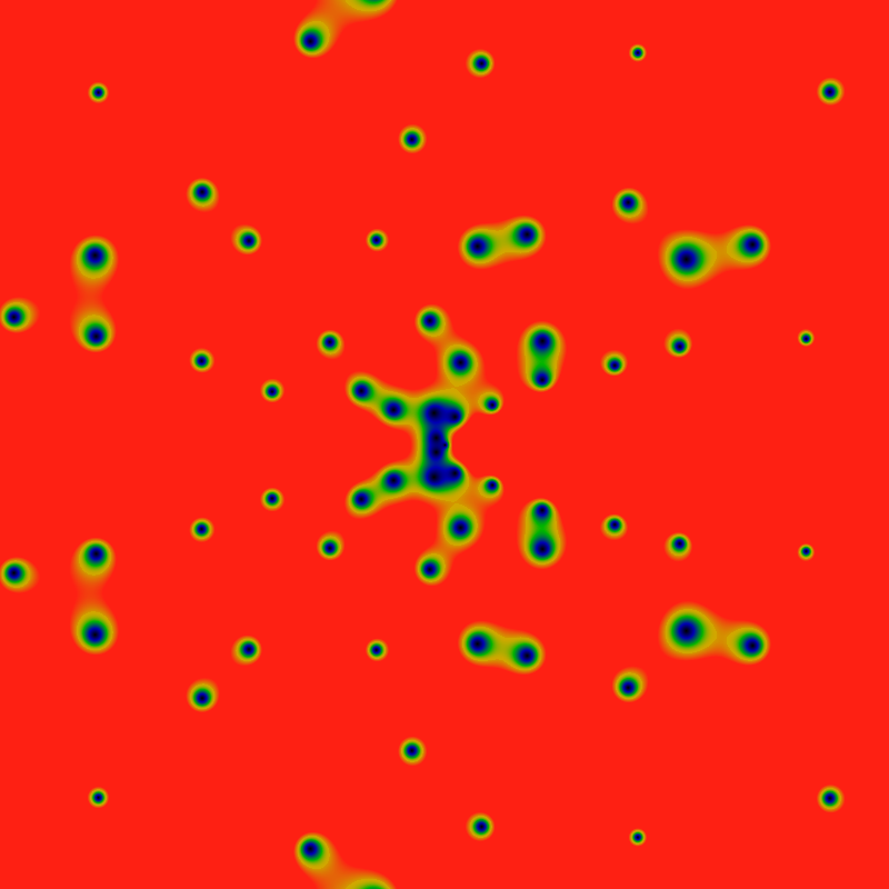
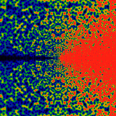
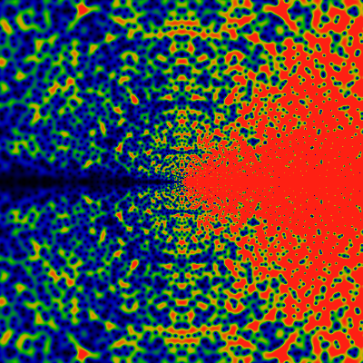
The zeros, again, but with the color maps scaled by 0.24.
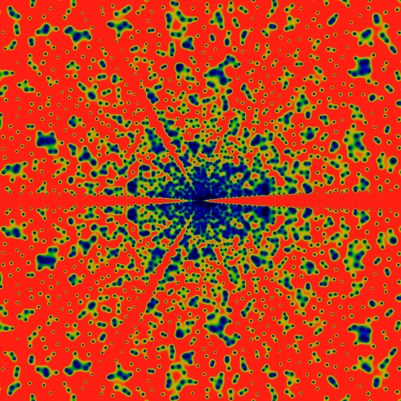
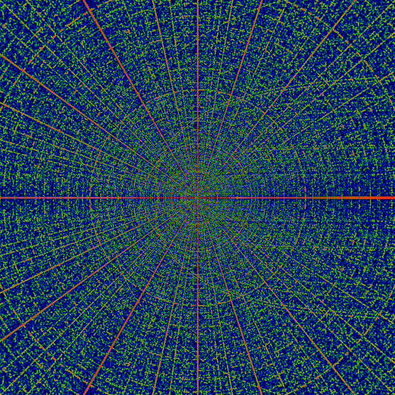
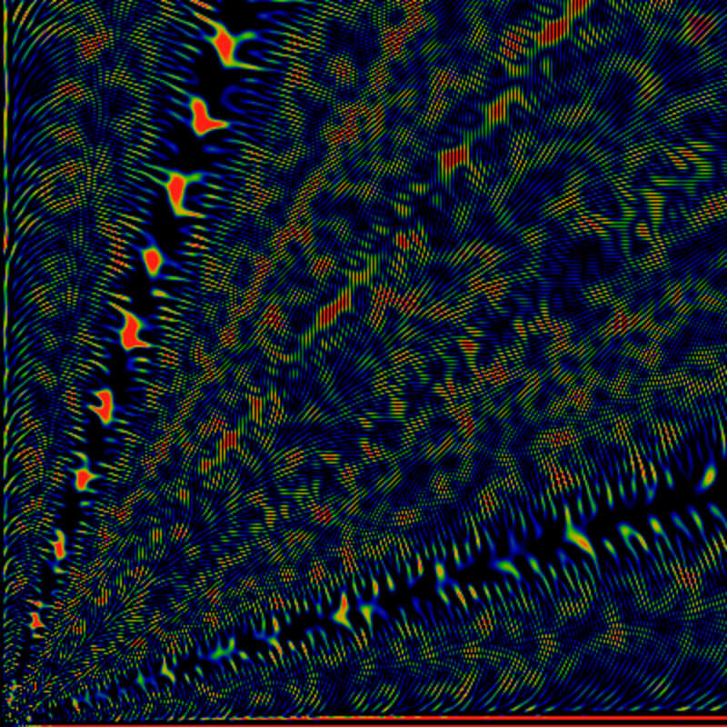
The zeros, again, but with the domain (x,y) ranging from -360 to +360. The big blue-black blobs to the right are five different zeros fairly close to each other. The color scale is adjusted so that green is about 0.2, and red is any value of 0.4 or greater.
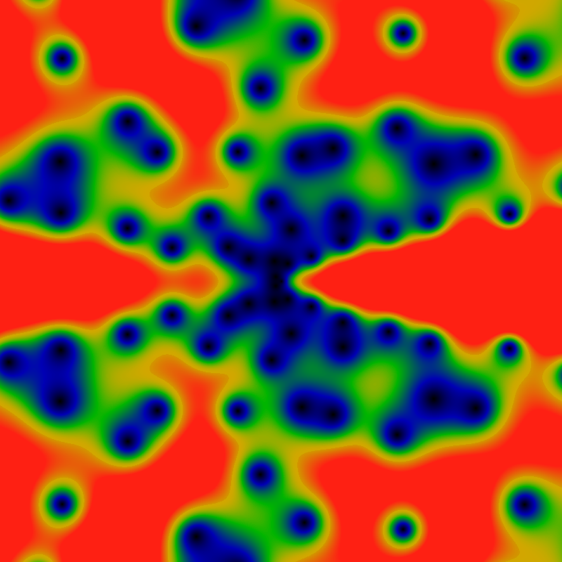
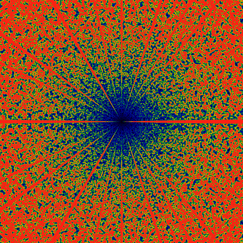
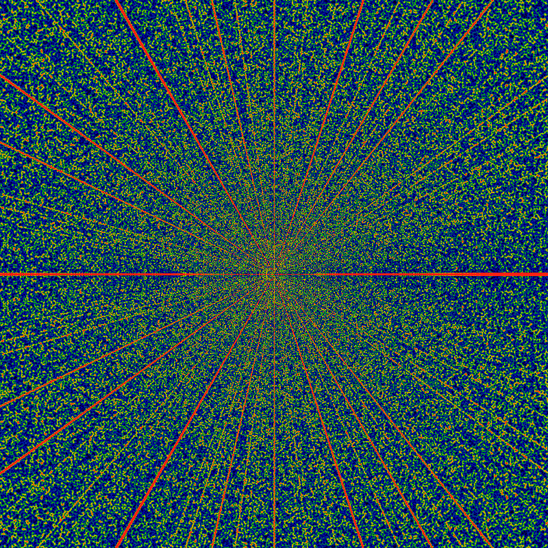
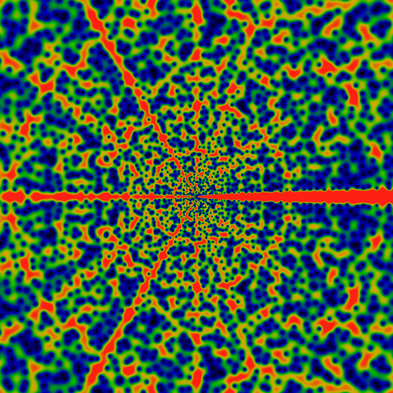
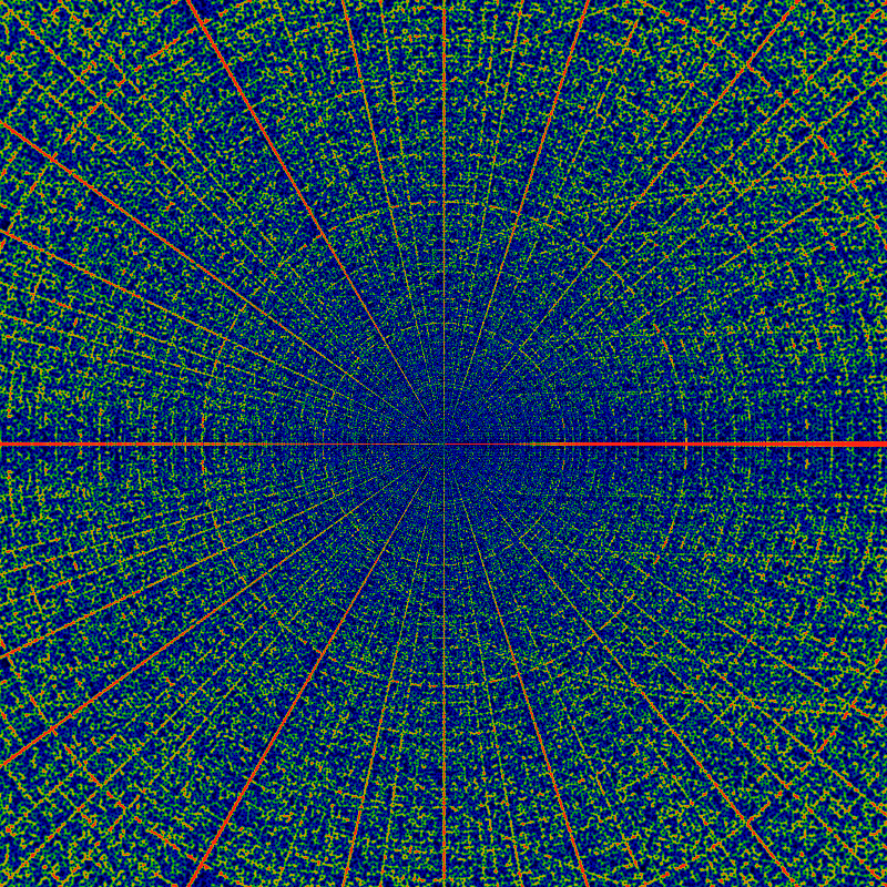
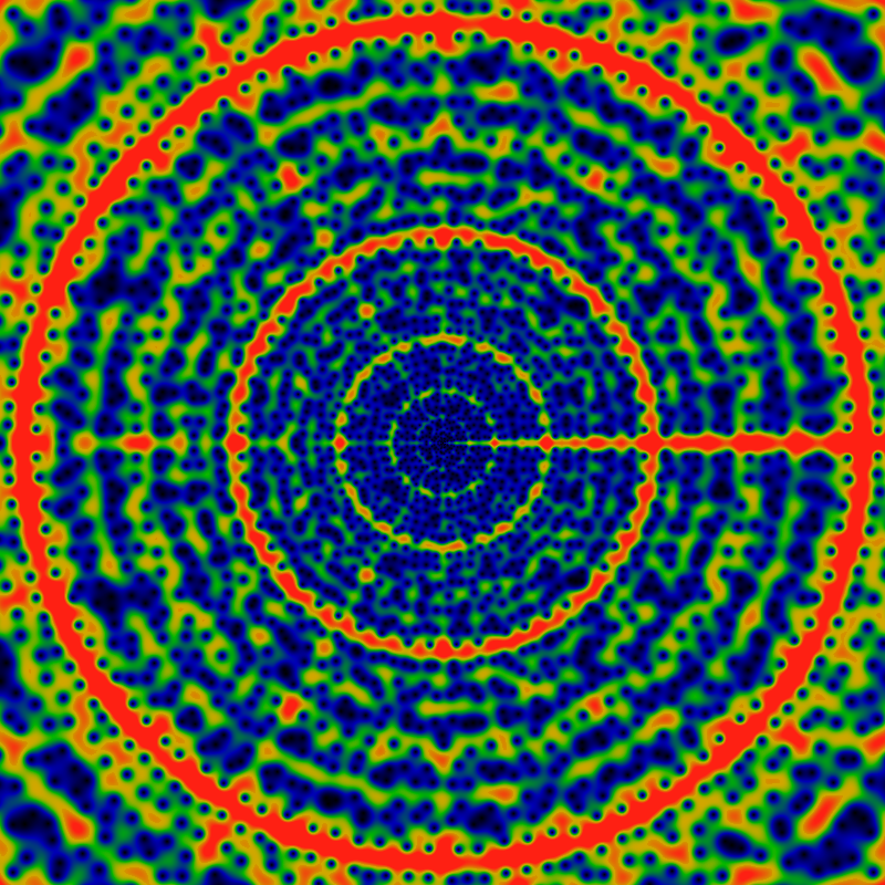
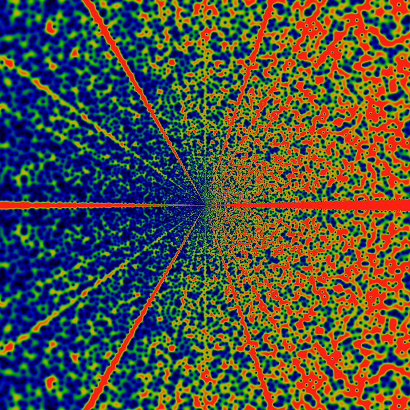
And again, but with the domain (x,y) ranging from -2160 to +2160. The colors are scaled to make the large-|z| zeros more clearly visible (values greater than 0.031 are red). This has the side-effect of exposing a new and interesting feature: rays! Lanes that are free of any zeros! Rays for the cyclic groups Z2 and Z3 are clearly visible, and with some peering, the rays for Z5 can be seen as well. There's a hint of Z7. Notably absent (or just hard to see?) are rays for Z4. This seems to lead to a natural conjecture that zeros never occur on rays for Zp, p prime.
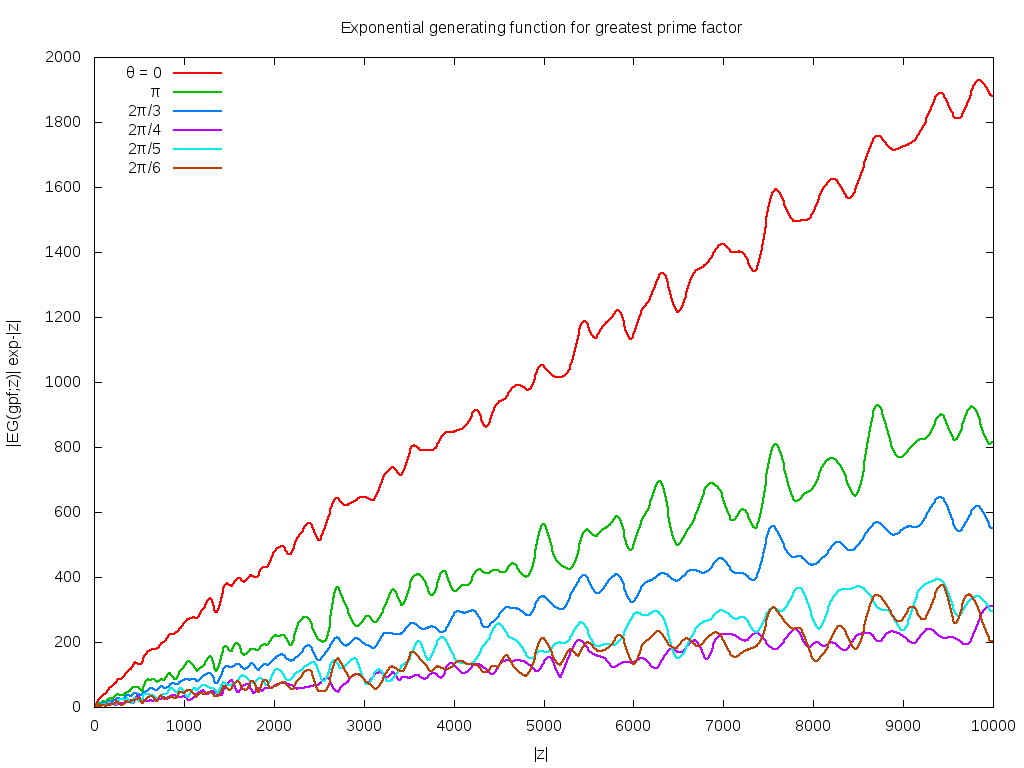
The above conjecture can be explored by taking slices along rays, shown below. It shows six slices, taken along the direction z=|z|exp iθ for θ=0, π, 2π/3, 2π/4, 2π/5, 2π/6 The leading divergence of exp|z| has been removed, leaving a divergence that seems to be about of order |z|/log|z|. Notable in this graph is that no zeros are visible along the rays for θ=2π/4 and θ=2π/6. This suggests the the above conjecture about primes was incorrect.
Most notable about this picture is the pronounced smooth oscillations along each ray. It's visually clear that the wavelengths get longer as |z| gets larger. Closer examination shows that the wavelength goes as the square-root of |z|.
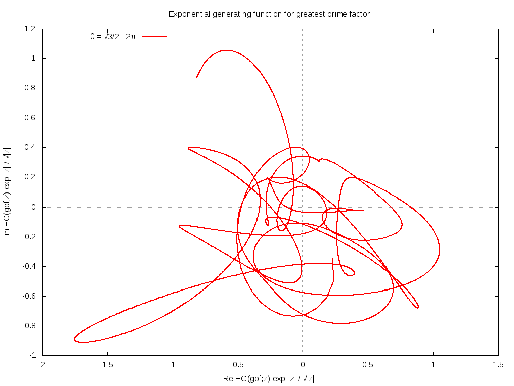
A similar exploration of rays directed along quadratic irrationals suggests that such rays pass very close to zeros on a number of occasions, but none actually pass through a zero. The below shows a phase plot of one such ray, graphing the real vs imaginary part of EG(gpf; z) for |z| running from 0 to 1000. The close passes are visible: recall that since the leading exponential scaling is removed, the close passes visualized here are indeed very close.
So where are the zeros located? Hard to say. The exploration of other angles, including simple fractions (without any factors of pi) suggests that these, too, manage to not hit any zeros, at least, not for |z| < 1000, although the ray for θ=1/3 really sure does come very, very close.
Here's a table of the 11 zeros nearest the origin. The coding is such that z=r exp(i π φ) = x + i y. Accuracy is good to about the last digit. Plouffe's inverter doesn't seem to know any of these numbers. They're presumably all some unknown transcendentals.
| r | φ | x | y |
|---|---|---|---|
| 1.5307945356883 | 0.78184092190433 | -1.1851209706937 | 0.96892734263997 |
| 4.0367224459103 | 0.39186518257935 | 1.3451122542394 | 3.8060216931609 |
| 4.5623453697754 | 0.60435053770449 | -1.4690131787199 | 4.3193744401079 |
| 8.3702116601813 | 0.22324068364269 | 6.3947066808728 | 5.4007564008976 |
| 8.4224011490127 | 0.80891465405978 | -6.9498220138446 | 4.7578162102767 |
| 11.344004468582 | 0.44048322811112 | 2.1087356654558 | 11.146285088604 |
| 13.460094569784 | 0.81744853194064 | -11.306557973367 | 7.3031426538461 |
| 15.804853981417 | 0.18788938300147 | 13.130504695764 | 8.7967753073744 |
| 16.909948423814 | 0.53886030109517 | -2.0592969204905 | 16.784089248133 |
| 19.238778607721 | 0.26037809273961 | 13.153182482454 | 14.040099461904 |
| 20.867068162569 | 0.76767832172763 | -15.551551998824 | 13.913438256922 |
Below is another table of zeros, this one for EG(ngpf; z), where ngpf(n) = n*gpf(n). That is, the gpf exponential series, except for (n-1)! in place of n!. Note that these are in the same general location as the above, except that they have moved inwards a bit.
| r | φ | x | y |
|---|---|---|---|
| 0.88022349562601 | 0.83295289206477 | -0.76176934606451 | 0.44102252283587 |
| 3.2375048946125 | 0.42458721923649 | 0.75986223121855 | 3.1470696420968 |
| 3.7441361185659 | 0.59817818048564 | -1.136602428757 | 3.5674486952574 |
| 7.4736771339129 | 0.23110162504623 | 5.5889493606786 | 4.9618035980621 |
| 7.511312297442 | 0.80582634942347 | -6.1565697810839 | 4.3030757558226 |
| 10.41426766772 | 0.44047959714246 | 1.9360237252942 | 10.232730974183 |
| 12.602613307375 | 0.81645934805374 | -10.564968103744 | 6.8707576832617 |
| 14.800600506967 | 0.19203401986558 | 12.187879585189 | 8.39722374263 |
| 15.997814072863 | 0.53774902696863 | -1.8927698515501 | 15.885448605531 |
| 18.340908478517 | 0.25911033247266 | 12.592535370681 | 13.334803213977 |
| 19.957065054996 | 0.768238424116 | -14.896747647415 | 13.280487759815 |
Note: the image runs out to a radius of 2160; to get the color map correct, the leading exponential divergence is removed, as is also a factor of log2(r)/r. In other words, rs(n) does have a different asymptotic behavior than gpf(n).
Perhaps the rays are due to the primes? One can consider a random distribution rps(n) having the property that 2 ≤ rps(n) ≤ n and also that rps(n) is prime. Below are EG(rps, z) for two such random sequences. No rays, but hints of rings! Curious! And also, an odd left-right symmetry! Clearly, more work can be done in this general area.
Some trees in a forest... photo by MIAN FAISAL.
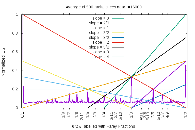
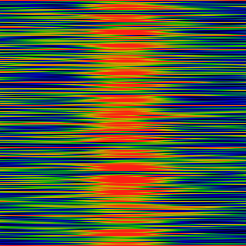
What are the angular locations of the zero-free lanes? These are shown below, and are labeled with Farey fractions, to show their positions, and with a bunch of Ley lines to demonstrate their heights. The graph was obtained by computing the absolute value |EG(gpf;z)| along radial slices. Plotting just one radial slice is noisy and indistinct, contradicting what is visually obvious. Thus, some noise cancellation is in order. This can be done by averaging together multiple radial slices; the figure below shows an average of 500 of them, taken near the radius r=|z| of about 16000. The zero-free lanes are the spikes. The tallest spike, at the angle of zero, was normalized to unit height; it sets the overall scale.
The spikes clearly correspond to the Farey fractions. A few seem to be missing: for example, 2/9 and 1/8 seem to be missing. Before jumping to conclusions, though, it might be the case that these are drowned in the noise. The heights of the spikes are very clearly predicted by straight lines with rational slopes, and are in Farey-order. The tallest spike is at 0/1, and by symmetry, also at 1/1. The first Farey fraction between these two is (0+1)/(1+1)=1/2, which is the second-tallest spike. Between these two is the next Farey fraction; it lies between 0/1 and 1/2 and so is (0+1)/(1+2) = 1/3 -- which is the location of the next tallest spike. After that, there are two Farey fractions: (0+1)/(1+3)=1/4 and (1+1)/(2+3)= 2/5. Argh! The pattern breaks down! Although the spike at 2/5 is indeed the next tallest, the spike at 1/4 is unexpectedly short. How is that even possible? Oh well.
Anyway, the two spikes at 1/5 and 2/5 seem to be of exactly the same height. The next row of the Farey triangle is 1/5, 2/7, 3/8 and 3/7. Clearly, there's a tall spike at 3/7, same height as 2/7 but taller than 2/8 and shorter than 1/5. So something throws off the regular patterning, even though the Ley lines clearly indicate that there is an exceptional amount of regularity.
Note that the heights are absolute heights, and not the heights relative to the noise floor. Presumably, working at more distant radii, and taking more averages would drop the noise floor; in the limit going to zero, I suppose.
The most notable aspect of this image is the narrowing of the rays. If one asked for the number of zeros in a pie-sliced wedge, and graphed that as a function of the angle, one would see a devil's-staircase type function. But, as this image shows, the treads on those stairs decrease in size as the radius of the circle increases. The rate is unclear; perhaps it goes as the square-root of the radius? That is, there are lanes that are completely free of zeros; these lanes get wider for larger radius, but at a sub-linear rate. They would have to, to make room for finite-width lanes for every rational! (A formula for the lane-width is discovered later, below.)
The widening of these zero-free lanes is one of the more interesting aspects of this image. Clearly, there is a suggestion of a ray for every rational. The simplest rationals have the widest lanes; but what, exactly, constitutes "simplest", here? If the rays are arranged according to widths, do they come in Farey-fraction order?
Also notable is a vague hint or suggestion of Moire patterning along the x-axis. Recall that Moire patterns occur when one regular (cyclic) grid pattern is superimposed on another, but shifted over. In this case, one regular pattern are the square pixels of the image; the other is the location of the zeros. The appearance of a Moire pattern is then strong evidence that the location of the zeros are not "random", but are correlated in some regular, cyclic way (as one moves from ray to ray). But of course it is: up above is a graph of six slices taken along a constant angle (six rays). These each show a characteristic oscillation with some very strong Fourier components. The Moire patterns are these same Fourier components, interfering with the characteristic pixel size.
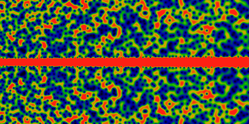
How real or illusory is the Moire patterning? Below shows a close-up, running along the domain 24000 < x < 48000 and -12000 < y < 12000. Again, there is a hint of yet more structure -- diagonal arrowhead/feather lines. Individual zeros are clearly distinguishable, and it is interesting how they line up so regularly, maintaining a uniform lane.
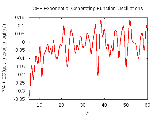
The asymptotic behavior of the generating function can be guessed at by numerical means. The graphs below show the re-scaled quantity -7/4 + EG(gpf; r) exp(-r) log(r) / r as a function of √r. The strong periodic oscillations are clearly visible. The rescaling hides just how small these oscillations are: So, for √r = 60, one has r = 3600 and r exp(r)/log(r) ~ 101566, and so the amplitude of the oscillations is 1566 orders of magnitude smaller than the function itself! OK, so the exponential divergence is obvious. What we have left is then r /log(r) ~ 440 so we're pulling out two orders of magnitude. That this does indeed seem to be the correct asymptotic scaling is reinforced by the graph that shows the same oscillations out to √r = 600. This corresponds to r = 360K and r /log(r) ~ 2.8 · 104, which is large! That the oscillations are happening around 7/4 = 1.75 is just a suggestion from the graph: closer numerical work suggests that the centerline is perhaps at 1.744.
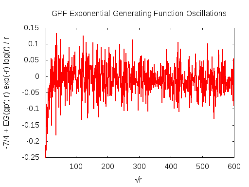
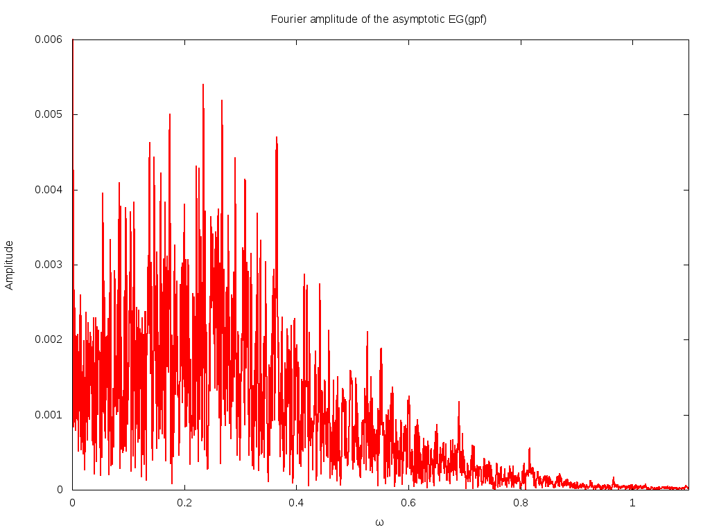
Perhaps the most notable feature of this graph is that, indeed, it looks very noisy: there is no obvious self-similar structure in it. Its hard to make out what the fall-off in frequency is: its perhaps cubic. In case you are wondering: no, this is NOT numeric noise; this can be most easily seen in the left figure above, where the oscillations are small and smooth; it is the Fourier components of this smooth graph that are not smooth. The calculations are performed with the Algorithmic 'n Analytic Number Theory multi-precision library (based on gnuMP); the results are verified by repeating the calculations at various different precisions.
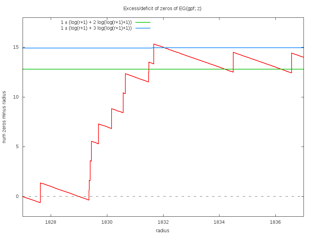
The graph below suggests that the strict bound is 1 ± [log(r+1) + Mlog(log(r+1)+1)] with equality holding at r=1 (there is one zeros inside of r=1). What's M? Good question. If you only graphed out to r=120, you might think that M=1 is a tight, but good bound. Not so, as it fails near r=123. So maybe M=2? Sure, that works out to about r=844, where it fails. So maybe M=3? Sure, that works out to about r=1832, where it fails. So maybe M=4? Sure, why not, the graph below supports that hypothesis.
Note that this linear dependence on the radius means that the density of zeros is decreasing as the square root -- the area of a circle goes as r2. Note that this graph is very compute-intensive to create: it represents several CPU-months of calculations.
Proving this bound may be hard; similar bounds are known to be equivalent to the Riemann hypothesis (examples include the bounds on Merten's conjecture (sums of the Mobius mu) and of Newton series expansions of Riemann zeta (Flajolet's paper with me), both of which have this characteristic square-root form). Of course, I have no clue if the zero-counting formula is equivalent to the Riemann hypothesis, but I would not be surprised.
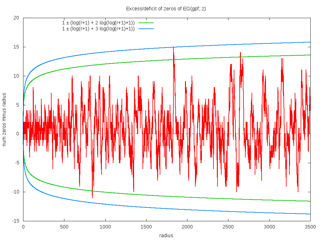
Below is a close-up of what happens near r=1832, where the count surpasses one of the hypothesized logarithmic bounds.
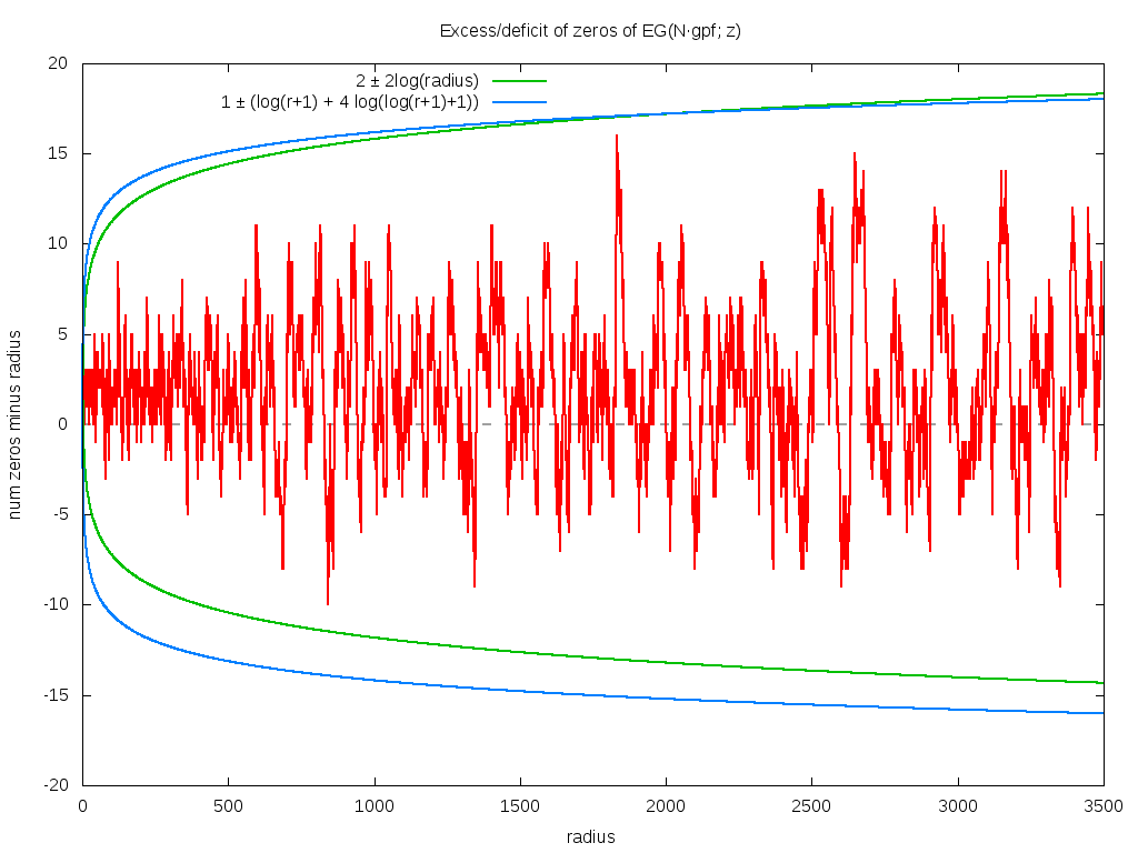
A very similar-but-very-slightly-different graph holds for EG(ngpf; z), where ngpf(n) = n·gpf(n) (the dot being simple multiplication). Two bounds seem acceptable, numerically. Aside from that suggested above, another possibility seems to be 2 ± log(r2), with equality holding at r=1 (there are three zeros inside of r=1, which is two more than expected). The logarithm is so slowly growing, that it's hard to say.
If you squint and scroll, you might notice that this and the previous
graph look suspiciously similar. Are they the same? No... but why so
similar? What's the point? For that, we need to look at a movie.
Oh, by the way: for any fixed radius, it seems that EG(ngpf; z)
always has about 2 to 6 (sometimes 8 or 10) more zeros than does
EG(gpf; z). It never-ever seems to have less.
There's another interesting thing: towards the end of the movie, on the negative x-axis, a pair of mirrored zeros coalesce into one (double) zero on the x-axis, and then split apart into two, in sequential order, one falling in before the other. Something similar also seems to happen on the ray 2π/5, although it is not clear if the two zeros actually coalesce before dropping in, or if they merely get close. At any rate, they start out roughly equidistant from the origin, but then fall in at sharply different times.
I've not verified the coalescing by hand. If that is what is really happening, then this appears to be a blatant violation that the lanes stay zero-free! This is surely something special and meaningful! Since it happens near frame 100 or so, its ... well, that's really a pretty big shift, for weird things to start happening. Wonder what it means.
I've never explored the action of shifts on exponential generating functions before; this behavior of radial inflow is a complete surprise to me. It turns out to not be unique to gpf; the exponential generating function of shifts of any of the random series discussed above also exhibit this kind of flow. Its presumably a well-known property of the exponential generating function; its just news to me.
The movie is 108 frames long, starting from a shift of zero. The domain is -100 < x,y < +100, and so almost every zero initially visible at the start of the movie has fallen into the origin by the end of the movie.
Clearly, there's a new feature visible here: rings! Concentric rings! Hard to tell, but, pulling out a ruler and eyeballing them, they seem to be located at powers of two: the outermost at a radius of 2048, then three more clearly visible at 1024, 512 and 256. Hard to tell, but there is a vague hint of another ring at 1536=3*512. And maybe yet many more rings! Wow! Who knew?
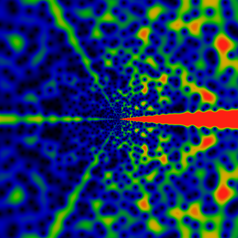
I lied. That's not the last image -- it pays off to keep making more. The below is the same as above, but over a domain ranging from -20K to +20K. Actually, its slightly different: it shows 0.005 EG(1/gpf; z) exp(-|z|) log5|z|, suggesting the asymptotic |EG(1/gpf; z)| ~ O(exp|z| log-5|z|) or thereabouts. The estimate of the logarithmic terms in the asymptotic behavior is a bit ambiguous. In this case, the asymptotic term was picked to give the appearance of a uniform color balance.
Newly visible are lines paralleling the positive x-axis, seeming maybe to curl around the origin in some vaguely parabolic way. There's a particularly large pseudo-parabolic orbit visible, coming in from the right, about 3/4th's of the way up, turning around the origin, and exiting abut 3/4th's of the way down (on the right, of course -- its easy to see, once you see it.)
As before, there are hints of Moire patterning along the x-axis, although this time, the scale of the picture is such that the individual zeros can still be distinctly made out. Therefore, the Moire patterns cannot be optical pixel-scale effects -- that is, its not an effect due to the finite size of the pixels -- it does not meet the criteria for the classical, canonical definition of the Moire effect in a computer graphics image. Instead, the Moire patterning seems to actually exist within the function itself! This suggests that perhaps the function itself can be decomposed as a sum of "layers", each layer consisting of a very regular oscillatory pattern, with only the sum of the patterns resulting in the apparent chaos of the image.
What are all these features? How are they to be described? What do they correspond to? One can't help but get the sense that this is the projection of some structure on some bundle, some structure built of sheafs and germs, but quite how to get that is unclear.
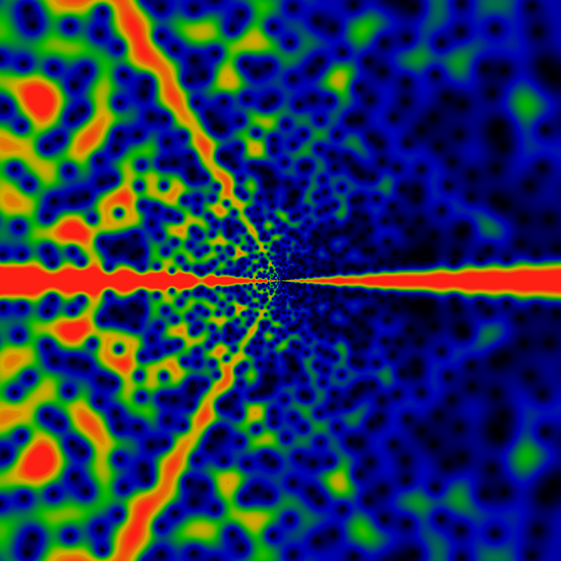
Below is same as above, except for a domain of -120K (= -1.2e5) to +120K. Note that there are parabola-like orbits facing to the left and to the right. Those aimed to the right are obviously visible; those to the left are extremely faint. There are also hints of other traceries, but its hard to say if these are merely optical, visual field effects or if they have some basis in mathematical reality.
This is my favorite, so here it is again, with a different asymptotic coloring scheme.
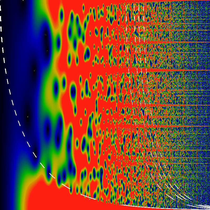
What are these parabolic-like orbits? Well, there's an alternate plot that makes curve-fitting easier. The below unwinds the the graph from around the origin, showing, much like the above, 1.6 EG(1/gpf; z) exp(-|z|) log1|z| log4[log(|z|+1)+1], except that here, z=r exp(iθ) with θ running along the vertical axis, from 0 to π. Along the horizontal axis, r is plotted on a logarithmic scale, so that r runs from 1 on the left to 65536 on the right. Superimposed on this figure are five hand-fitted dashed white lines. One tries to capture the edge of the root-free zone. This line is given by sin θ/2 = 1/√r. Note the radical. Careful examination shows that at least a few zeros appear on the wrong side of this line -- the shape seems to be only approximate. Four more lines try to fit the pseudo-parabolas. The fits are OK on the large-r asymptotic region, but poor in the small-r region. The four that are drawn are given by
| 768/r = sin θ/2 |
| 1200/r = sin θ/2 |
| 1500/r = sin θ/2 |
| 1948/r = sin θ/2 |
| 7200/r = sin θ/2 (not drawn) |
What happened to the circles? They should be vertical lines in the above! Well, they are still there, just too narrow to be visible in the above. They do become visible, below: five evenly spaced vertical lines, using the same mapping and logarithmic scaling as above. The domain of r is from 1024 on the left to 65536 on the right, so the five vertical lines correspond to r=2048, 4096, 8192, 16384, and 32768, respectively. Otherwise, there is nothing particularly new in this image; everything visible here is visible in earlier images.
Just how thin are these vertical lines? The image below is a closeup of the image above: in this case, r runs from (32768-650) to (32768+650). Eye-balling the red strip, it seems maybe 350 units wide -- so maybe a width of √32768=362 is a decent wild guess. Is this vertical stripe really zero-free? Hard to tell from this picture. There are lots of blue smears -- there are about 650 zeros in this image (as demonstrated earlier, there are about r zeros inside a circle of radius r; the width of this image is 650+650, but the height is only π, not 2π.) Fiddling with the color-map helps isolate some of these a bit more clearly, and it seems like there might be dozen or two zeros actually within the red stripe, rather than all the blue being just a smear from outside the stripe.
As above, but for the region 0 < x,y < 4000. Should not be any need to point out that Moiré patterning is very sensitive to the sampling frequency.
As above, but for the region 0 < x,y < 8000.
One may also consider a very similar sum, using the falling Pochhammer symbol, instead of the rising one. This symbol is given by (z)n = z(z-1)(z-2)...(z-n+1). The resulting image appears below, it is of FPG(gpf,z) exp(-2 √ |z|) / |z| with normalization exactly as given and coloration as always.
Some of the first few zeros for the rising Pochhammer generating function are shown below. Note that the first two lie precisely on the real axis. The others do not seem to occur at any low rational angle (the column φ shows the angle in units of pi, thus a value of φ of one indicates the negative x-axis), although the next few seem to try to get close to the 3rd roots of unity, and the one after that the 6th root of unity. After that, there is no clear progression. As before, they are presumably transcendental, rather than, for example, quadratic irrationals, or some such.
| r | φ | x | y |
|---|---|---|---|
| 1.3949092398684 | 1 | -1.3949092398684 | 0 |
| 4.5626759564288 | 1 | -4.5626759564288 | 0 |
| 10.245898379007 | 0.64420879547681 | -4.4846874842696 | 9.2122750589292 |
| 24.83352515618 | 0.63379620727208 | -10.133683877231 | 22.671842068058 |
| 55.576607747775 | 0.3205855915997 | 29.693058011758 | 46.979587425396 |
| 72.25879634152 | 0.8121672651601 | -60.038996469216 | 40.207618080342 |
| 117.75420722502 | 0.46759200907347 | 11.968172804434 | 117.1444243612 |
| 192.15199916793 | 0.81693429156798 | -161.24015864602 | 104.51795072638 |
| 201.03591391007 | 0.25107689390384 | 141.67211584758 | 142.63397306717 |
| 285.6352301736 | 0.54737231184267 | -42.35277394865 | 282.47783498034 |
| 364.85530526812 | 0.27307016022456 | 238.63224457153 | 275.99645945745 |
| 442.19734166307 | 0.78730029361836 | -347.09323384104 | 273.97951747467 |
| r | φ | x | y |
|---|---|---|---|
| 0.72183600549901 | 0.49137876622082 | 0.019548108331473 | 0.72157126487647 |
| 10.360150450484 | 0.45106261529342 | 1.5865160932827 | 10.237953117808 |
| 23.302941560009 | 0.47588077521583 | 1.7640394756877 | 23.236076477697 |
| 57.987569085342 | 0.7605584350114 | -42.340693875438 | 39.621002139948 |
| 67.48077369795 | 0.26157732931857 | 45.949442919987 | 49.419667281528 |
| 122.32995335662 | 0.40689342952179 | 35.273809336995 | 117.13400814063 |
| 168.26853286447 | 0.78918215559082 | -132.69280305254 | 103.4742439954 |
| 224.60980862841 | 0.22477866727782 | 170.89602763141 | 145.75360672003 |
| 281.86194385292 | 0.50767619198356 | -6.7965739748906 | 281.77998859881 |
| 393.67913951173 | 0.2492135681373 | 279.06010117129 | 277.68457793146 |
| 410.84081343407 | 0.76652914265676 | -305.19542443344 | 275.03804625552 |
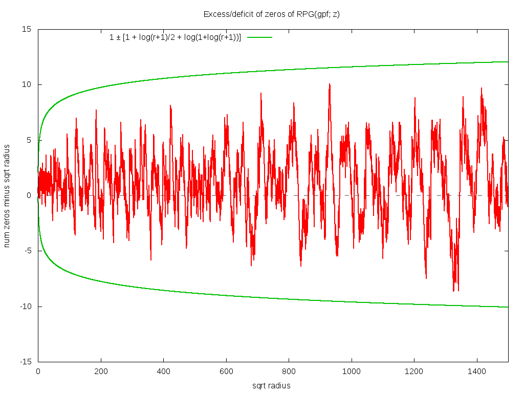
How many zeros are there? As before, we have the curious similarity: the bound on the rate of divergence of the function gives the count of the zeros. Thus, asymptotically RPG(gpf; z) seems to go roughly as O(|z| exp (2 sqrt|z|). The number of zeros inside a circle of radius |z| appears to be given by 1 + √ |z| and the error of this approximation is bounded by ± [1+log(1+|z|)/2+log(1+log(1+|z|))], as the graph below shows. This bound appears to be tight; nothing tighter seems to work. Note that this bound extends all the way to |z|=0 -- that is, it is not violated at small |z|.
The use of exponential generating functions with almost any classical arithmetic function arising in number theory (such as the divisor function, the Euler totient, the prime counting function, etc.) is very nearly unheard of, and tackling the greatest prime factor in this way is unique. Why would that be so? Because there are no known results for the exponential generating function in this setting. This is in sharp contrast to the Dirichlet generating function (i.e. the Dirichlet series) or the Lambert generating function (Lambert series) which have a vast number of identities commonly presented in undergraduate number theory courses. (See e.g. Apostol, "Introduction to Analytic Number Theory", Springer.)
The visually apparent symmetries in the images here makes it quite clear that there is some sort of distorted modular symmetry at work, apparent just out of easy reach. The figures here whet the appetite. Perhaps a proper theory of these figures would start with something simpler than the greatest prime factor function: certainly the divisor function and the Euler totient function appear to be far more regularly patterned, when passed through the exponential generating function. But even then, although there is a tremendous visual regularity to those figures, it still seems impossible to obtain closed form solutions. So the best one can do for now is to stare in wonder.
Initial version: April 2016. Revised version: October 2016

Greatest Prime Factor
by Linas Vepstas is licensed under a Creative Commons
Attribution-ShareAlike 4.0 International License.