This paper is part of a set of chapters that explore the relationship between the real numbers, the modular group, and fractals.
Linas Vepstas <linas@linas.org>
Date: 12 October 2004 (revised 15 November 2004)
This paper is part of a set of chapters that explore the relationship between the real numbers, the modular group, and fractals.
Given a real number
![]() , a sequence of integers
, a sequence of integers
![]() can be found that define its continued-fraction expansion:
can be found that define its continued-fraction expansion:
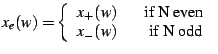
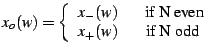
Given a rational ![]() and an arbitrary complex number w, define new
sequences:
and an arbitrary complex number w, define new
sequences:
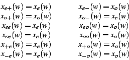
There is also an even-odd symmetry for ![]() that we should be aware
of, as it plays another important role in the theory. As we point
out above, for any given sequence, there is a + and a - generalization.
But what if the sequence is already
that we should be aware
of, as it plays another important role in the theory. As we point
out above, for any given sequence, there is a + and a - generalization.
But what if the sequence is already ![]() and we choose the - expansion?
Then we get
and we choose the - expansion?
Then we get
If one needs to take differences, e.g. for derivatives, the even-odd
expansion is more useful: Define ![]() and
and ![]() as follows:
as follows:
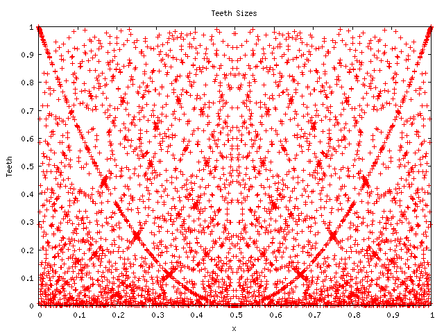
Let use define the gap as
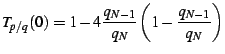
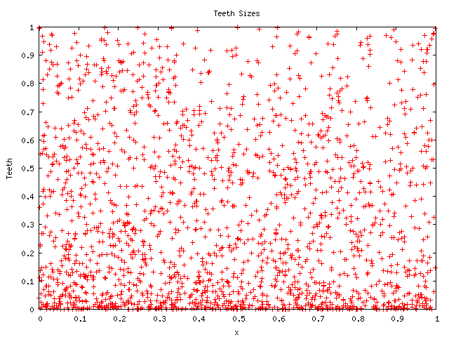
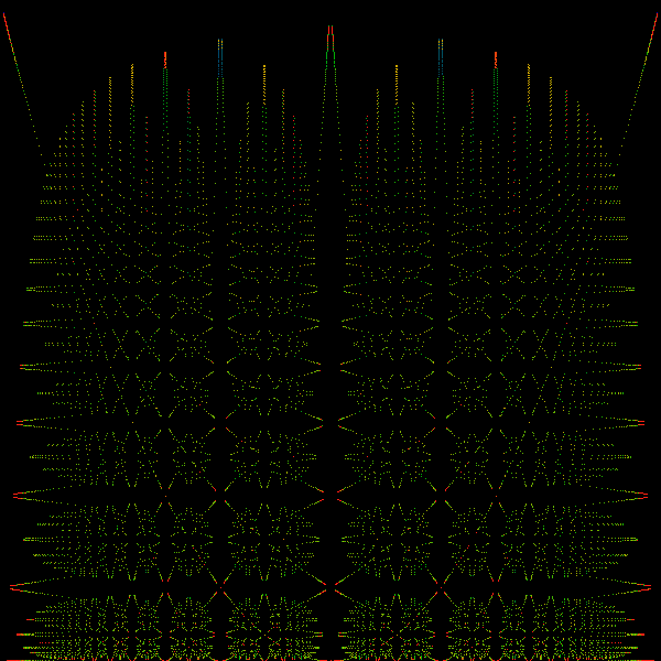
The teeth at first appear to be random: below follows a scatter-plot
showing ![]() for a thousand randomly generated small-ish rationals.
for a thousand randomly generated small-ish rationals.
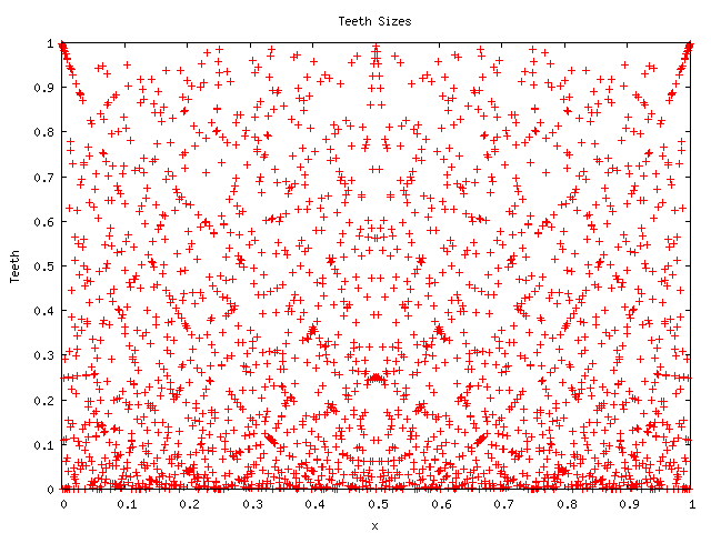
However, closer examination reveals some surprising details. Here's
the same picture, but this time showing only the rationals
![]() (all rationals with numerator between 1 and 719 and denominator of
720:
(all rationals with numerator between 1 and 719 and denominator of
720:
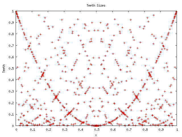
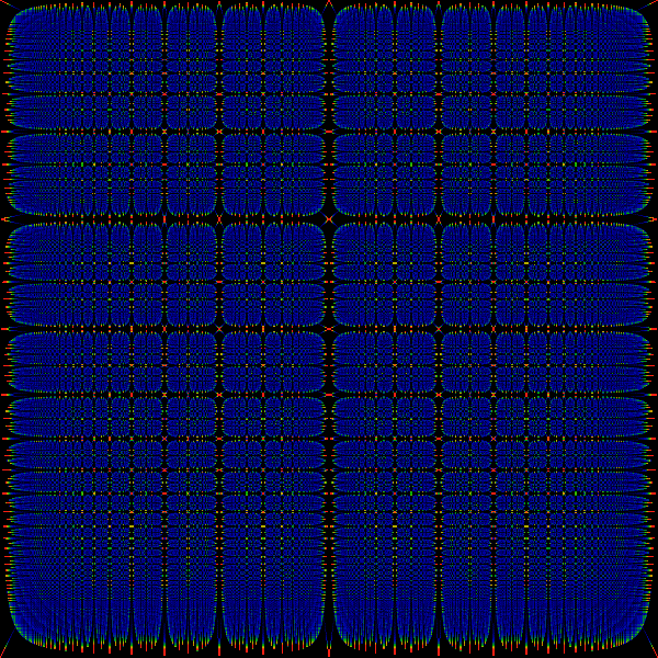
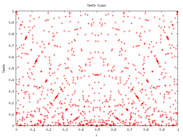
Note that 720 = 6! (six factorial) and that similar but denser images
appear for higher factorials: Here's one for ![]() that is,
that is,
![]() :
:
Notice that a Moire pattern of fringes seems to be forming at ![]() .
The appearance of various parabolas at various locations seems to
indicate that there are some sort of curious algebraic relationships
between the rationals that are worth exploring. The factorial in the
denominator seems important: the picture for the denominator
.
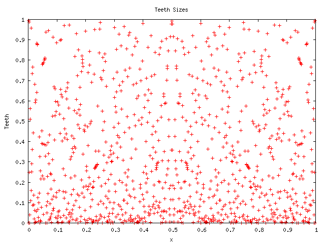
The appearance of various parabolas at various locations seems to
indicate that there are some sort of curious algebraic relationships
between the rationals that are worth exploring. The factorial in the
denominator seems important: the picture for the denominator
![]() blurs out the features, and mostly looks much more random, as shown
below:
blurs out the features, and mostly looks much more random, as shown
below:
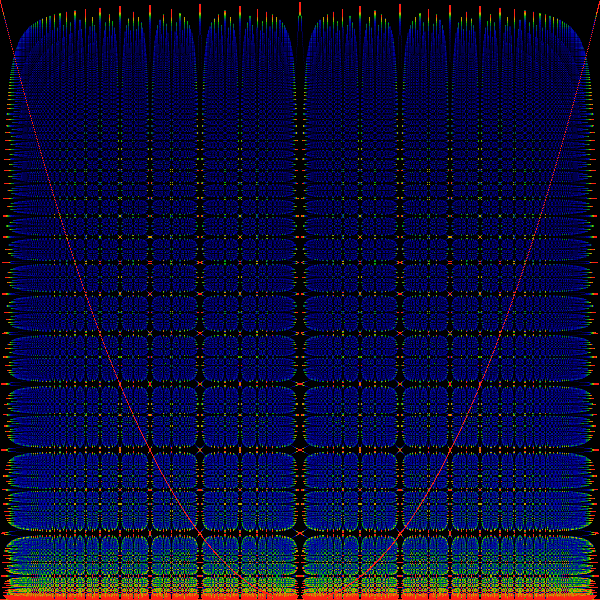
Now that we know what sort of pattern to look for, we can find the cross-bars in this picture, for a denominator of 1024:
The analogous picture for a denominator consisting of powers of 3 is less distinct. Pictures for prime denominators appear considerably more random, although containing hints of a different kind of structure. For example, here is a picture with denominator 1023:
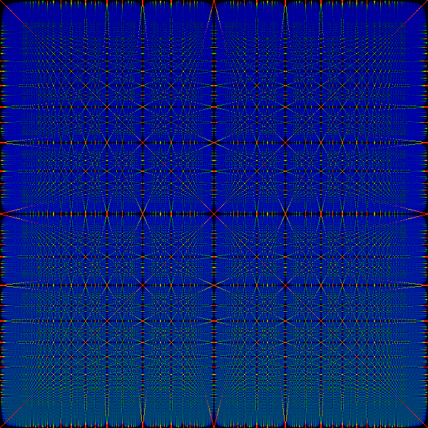
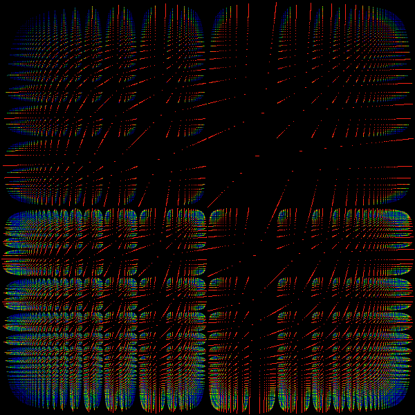
The next picture below is a scatter-plot showing all rationals with denominators less than 200. This now clearly exhibits a fantastic self-similar fractal latticework:
We will recognize in later chapters that these curves correspond to
hyperbolic maps of the unit interval back onto itself, generated by
elements of the modular group
![]() acting on binary
trees. It would be interesting to specify the shapes of all the various
bifurcating curves that seem to appear in this latticework, and to
give the algebraic equations whose solutions are plotted above. Note
that because a curve can seemingly bifurcate into another curve in
many places, enumerating all of them would be a trick.
acting on binary
trees. It would be interesting to specify the shapes of all the various
bifurcating curves that seem to appear in this latticework, and to
give the algebraic equations whose solutions are plotted above. Note
that because a curve can seemingly bifurcate into another curve in
many places, enumerating all of them would be a trick.
There are more interesting things to be seen, but first we should
provide a simpler expression for
![]() at
at ![]() . Recall that
for any fixed rational
. Recall that
for any fixed rational ![]() , that
, that
![]() is of the form
is of the form
![]() for some positive integers
for some positive integers ![]() . For any given, fixed
. For any given, fixed ![]() ,
there exists an
,
there exists an
![]() such that there are no poles in
such that there are no poles in
![]() in the disk of radius
in the disk of radius ![]() around
around ![]() (Homework: prove this),
and thus its analytic on this disk. This justifies an expansion in
(Homework: prove this),
and thus its analytic on this disk. This justifies an expansion in
![]() ; we'll give an exact expression in a later section, showing that
these manipulations are safe. For the continued fraction
; we'll give an exact expression in a later section, showing that
these manipulations are safe. For the continued fraction
![]() we write the
we write the ![]() 'th partial convergent as
'th partial convergent as
![]() which obeys the recurrence relation
which obeys the recurrence relation
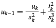
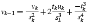
![]() . Substituting, we get the explicit recurrence relations for each
term:
. Substituting, we get the explicit recurrence relations for each
term:
For reference, overdrawn over the image is the parabola. The vertical
black stripes occur at the Farey numbers, and appear to be ordered
in size according to the Farey tree (i.e. the largest stripe
is at ![]() , the next largest at
, the next largest at ![]() ,
, ![]() and the next
smaller ones at
and the next
smaller ones at ![]() and
and ![]() etc.). The progression
of the horizontal bands are clearly related to the Farey tree through
the parabola. Since the parabola gives a rational out when fed one
in, we see that we've discovered a different tree of rationals that's
related to the Farey tree. One can see that any ratio of polynomials
will this give a tree of rationals. We discuss the Farey Tree (or
Stern-Brocot Tree) in a different chapter.
etc.). The progression
of the horizontal bands are clearly related to the Farey tree through
the parabola. Since the parabola gives a rational out when fed one
in, we see that we've discovered a different tree of rationals that's
related to the Farey tree. One can see that any ratio of polynomials
will this give a tree of rationals. We discuss the Farey Tree (or
Stern-Brocot Tree) in a different chapter.
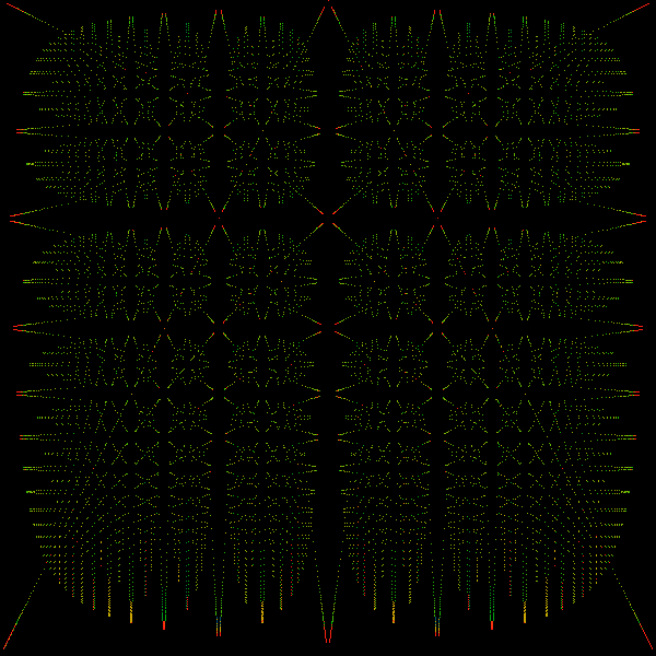
The filigree pattern exists only for small rationals. If we start sampling larger rationals, the distribution becomes smooth. The picture below shows a random sampling of rationals with denominators less than 2 million. The image is a bit grainy because the sample size is not large enough; the graininess goes away with larger sample sizes.
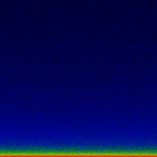
This picture tells us something that is surprising: this function
is space-filling and dense; it has no holes or islands; it has a fractal
measure of 2.0. Even in the land of fractals, this is fairly unusual,
as this function is, after all, not some self-similar curve, but rather
a 'plain-old' map from the unit interval to the unit interval. By
'dense', I mean the traditional Cauchy-sequence notion of density:
for any real values
![]() and positive
and positive
![]() ,
we can find a rational
,
we can find a rational ![]() such that
such that
![]() and
and
![]() . Of course, a computer
generated picture is not a proof, but a proof is straight-forward,
and is discussed below. I am not aware of any other map that has this
property.
. Of course, a computer
generated picture is not a proof, but a proof is straight-forward,
and is discussed below. I am not aware of any other map that has this
property.
The distribution of the gaps ![]() can be easily found to be
can be easily found to be
![]() which is sharply peaked at
which is sharply peaked at ![]() : this is the thin
red stripe at the bottom of the above picture. This distribution is
due to the Jacobean of a parabola, which we derive below.
: this is the thin
red stripe at the bottom of the above picture. This distribution is
due to the Jacobean of a parabola, which we derive below.
One can get a better idea of the behavior of ![]() by graphing
it, as a function of
by graphing
it, as a function of ![]() , for a number of representative values of
, for a number of representative values of
![]() . From the above analysis, we should suspect that for
. From the above analysis, we should suspect that for ![]() ,
the leading
,
the leading ![]() terms are of magnitude
terms are of magnitude ![]() which would make
it hard to directly compare different values of
which would make
it hard to directly compare different values of ![]() So instead,
we introduce a 'normalized' variant:
So instead,
we introduce a 'normalized' variant:
![]() and similarly
and similarly
![]() . This is done below, for 200 evenly
spaced values of
. This is done below, for 200 evenly
spaced values of ![]() . On the horizontal axis is
. On the horizontal axis is ![]() running from
0 to 1, and along the vertical axis,
running from
0 to 1, and along the vertical axis, ![]() , from 0 at bottom to 1 at
top:
, from 0 at bottom to 1 at
top:
Clearly, it can be seen that
![]() is a monotonically increasing
function of
is a monotonically increasing
function of ![]() , which follows easily by examining the partial sums:
if
, which follows easily by examining the partial sums:
if ![]() then
then
One finds a mirror symmetry between the even and odd forms:
![]() ,
which is also not quite obvious, given the construction. Its is clear
from this picture that the leading
,
which is also not quite obvious, given the construction. Its is clear
from this picture that the leading ![]() and
and ![]() terms dominate.
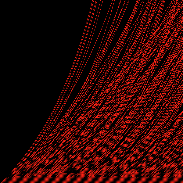
We can guess at the form of these terms: we define
terms dominate.
We can guess at the form of these terms: we define
![]() and graph it below, exposing the randomness of the cubic and higher
terms directly.
and graph it below, exposing the randomness of the cubic and higher
terms directly.
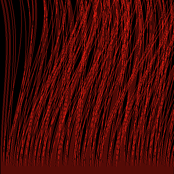
The seeming parallel-ness of some trajectories is an optical illusion, due to the pixelization of the picture. There are more pictures, with a greater number of strands, at the Gap Room http://www.linas.org/art-gallery/farey/gap-room/gap-room.html.
The size of the gap can be given an exact expression in terms of the convergents of the continued fraction. Performing this exercise will help explain some of the fractal behavior seen in the previous sections.
One gets the convergent of a continued fraction by evaluating the
fraction only up to the ![]() 'th term, and expressing it as a ratio
'th term, and expressing it as a ratio
![]() . The convergents can be expressed recursively:
. The convergents can be expressed recursively:
The distribution density
![]() of the gaps on the unit square
can now be understood in terms of the above parabolic formula, as
a change-of-variable from the underlying distribution of
of the gaps on the unit square
can now be understood in terms of the above parabolic formula, as
a change-of-variable from the underlying distribution of
![]() .
Numerically, we can confirm that this distribution is, in a certain
sense, perfectly uniform on the half-unit square. Now that we understand
that the more fundamental quantity with regard to distributions is
.
Numerically, we can confirm that this distribution is, in a certain
sense, perfectly uniform on the half-unit square. Now that we understand
that the more fundamental quantity with regard to distributions is
![]() , lets repeat some of the earlier graphs. These are shown
in
, lets repeat some of the earlier graphs. These are shown
in ![]() and
and ![]() .
Visually, they don't differ much from thier earlier analoguous, except
for an effective rescaling of
.
Visually, they don't differ much from thier earlier analoguous, except
for an effective rescaling of
![]() . Nonetheless, they are
presented here for reference.
. Nonetheless, they are
presented here for reference.
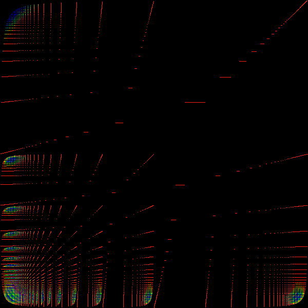
The figure above shows the distribution of the ratio of the final
two convergent denominators
|
The figure above shows the distribution of the ratio of the final
two convergent denominators
|
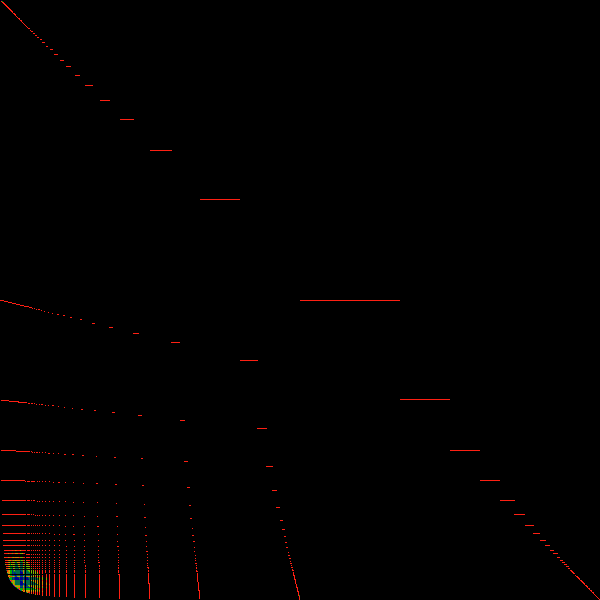
It is of some interest to examine distribution of other convergents. This section reviews some of these.
The figure above shows the distribution of the ratio of the pre-final
two convergent denominators
|
The figure above shows the distribution of the ratio of the pre-final
two convergent denominators
|
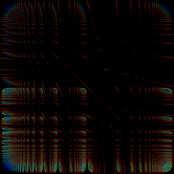
The figure above shows the distribution of the ratio of the two convergent
denominators
|
The figure above shows the distribution of the ratio of the two convergent
denominators
|
The figure above shows the distribution of the ratio of the two convergent
denominators
|
The figure above shows the distribution of the ratio of the two convergent
denominators
|
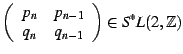
The relationship between convergents
![]() implies that the matrix
implies that the matrix
The computer efforts at first seem to paint two contradicting interpretations about the distribution of the gaps. For small denominators, there seems to be a detailed and fine structure; yet, for large denominators, this structure seems to blur away, and one gets the impression of a perfectly uniform distribution. In fact, both conclusions are correct. Each of the pictures above and below were created with a uniform pixel size: 600 pixels dividing up the interval 0 to 1. For small denominators, each pixel may contain only one gap, and maybe none; for large denominators, each pixel may represent the average of dozens or hundreds of gaps. It seems reasonable to conclude that the structure of horizontal and vertical bars is in fact scale-invariant, and persists down to infinitesimal scales. Looking at large-denominator distributions with only 600x600 pixels effectively blurs all the structure away. Thus, on a coarse-grain, the distribution of the gaps appears to be perfectly random; a finer choice of binning, while holding denominators fixed, would lead to pictures of detailed structures at finer levels, and so on.
Thus, in order to talk about the gaps for ``all rationals'', one has two competing limits that give different answers. In one case, we take the size of the pixels smaller and smaller, and find, for any fixed scale of denominators, that there is a highly fractal filigree. In the other case, we hold the size of the pixels fixed, and take the limit of larger and larger denominators, and find a perfectly uniform distribution. It seems impossible to define the distribution ``in and of itself'' without resorting to talking about pixels at some point.
The incredible 'randomness' of the distribution, as well as its Cauchy-sequence-density on the unit square can now be easily understood. To do this, consider the iteration of the map
Lets try to restate the paradox. We would like to be able to say,
that, when considering the entire set of reals on the unit interval,
that, when examining the ![]() 'th binary digit in the expansion, that
'th binary digit in the expansion, that
![]() 'th digit is completely random, and is uniformly distributed (equipartition
of probability), with the probability of the digit being 0 being 1/2
and the probability of it being 1 is also 1/2. But of course, this
statement is patently false, and therein lies the paradox. We can,
of course, trivially and exactly predict the
'th digit is completely random, and is uniformly distributed (equipartition
of probability), with the probability of the digit being 0 being 1/2
and the probability of it being 1 is also 1/2. But of course, this
statement is patently false, and therein lies the paradox. We can,
of course, trivially and exactly predict the ![]() 'th digit, as the
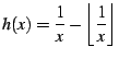
Bernoulli process is completely deterministic. The
'th digit, as the
Bernoulli process is completely deterministic. The ![]() 'th digit is
trivially
'th digit is
trivially
![]() and the graph of
and the graph of ![]() is a square-toothed comb. One has this
problem even for
is a square-toothed comb. One has this
problem even for ![]() getting very large, and approaching infinity:
the comb remains uniform and entirely ``predictable'' no matter
how large
getting very large, and approaching infinity:
the comb remains uniform and entirely ``predictable'' no matter
how large ![]() gets.
gets.
I suppose there are two ways out of this paradox. One way out is to
say something like ``Yea, Verily, Chooseth two Irrationals whose
Binary Expansions are Completely Uncorrelated'', which sounds like
an invocation of the Axiom of Choice. Indeed, the set of computable
numbers is countable, and is of measure zero on the real number line.
In order to compute the ![]() 'th digit of
'th digit of ![]() , one must somehow already
'know'
, one must somehow already
'know' ![]() . Since the set of of unknowable numbers has measure one
on the unit interval of reals, one arguably must 'choose' if one is
to get a truly 'random' number. Thus, we can anchor the concept of
randomness of bit-sequences of the binary expansion of real numbers
in the concept of Turing-uncomputable numbers and the Axiom of Choice
for choosing one of these unknowable numbers. This is cleary dangerous
territory, and somewhat tangled as a definition of randomness.
. Since the set of of unknowable numbers has measure one
on the unit interval of reals, one arguably must 'choose' if one is
to get a truly 'random' number. Thus, we can anchor the concept of
randomness of bit-sequences of the binary expansion of real numbers
in the concept of Turing-uncomputable numbers and the Axiom of Choice
for choosing one of these unknowable numbers. This is cleary dangerous
territory, and somewhat tangled as a definition of randomness.
The other way out of the paradox is far more mundane, and seems constructive,
and that is to apply shop-worn statistical methods. After all, chaos
occurs in numerical simulations, on finite and computable sets, and
not in set-theoretical limits. Chaos is a computational phenomenon.
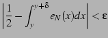
What we can say is that for any given real ![]() and
and ![]() and
and
![]() , one can always find an integer
, one can always find an integer ![]() such that the
average value of
such that the
average value of ![]() approaches 1/2 on the interval: that is,
there exists an integer
approaches 1/2 on the interval: that is,
there exists an integer ![]() such that
such that
Now, to move the conversation back to the iterated continued fraction map, and that proof.
The work of Cantor shows that the cardinality of
![]() is the same as that of
is the same as that of
![]() , namely
, namely
![]() . This implies
that the points of
. This implies
that the points of
![]() can be enumerated by
can be enumerated by
![]() .
Space-filling curves such as those of Peano or Hilbert can be used
to develop that enumeration. However, these curves have a locality
property, in that if two points are close to each other in
.
Space-filling curves such as those of Peano or Hilbert can be used
to develop that enumeration. However, these curves have a locality
property, in that if two points are close to each other in
![]() ,
then the points that they enumerate in
,
then the points that they enumerate in
![]() are also
close to each other. This is by construction, of course: the curves
of peano or Hilbert are inherently continuous. We can, for example,
graph the distance of the Hilbert curve from the the x-axis as a function
of the parameter that takes us along the curve. By construction, this
is a continuous curve, and it is *not* space-filling.
are also
close to each other. This is by construction, of course: the curves
of peano or Hilbert are inherently continuous. We can, for example,
graph the distance of the Hilbert curve from the the x-axis as a function
of the parameter that takes us along the curve. By construction, this
is a continuous curve, and it is *not* space-filling.
By contrast, the gap function is not a curve; by construction, it seems to be discontinuous everywhere.
The cause of the principal parabola seen in the pictures is now also clear. Blah Blah Blah write this section too.
The main parabola that is visible is at
![]() ,
which we can solve for directly to obtain
,
which we can solve for directly to obtain
![]() and
and
![]() . Recalling that by definition,
. Recalling that by definition,
![]() ,
we find that the rationals on the main parabola are given by
,
we find that the rationals on the main parabola are given by
![]() and
and
![]() . Blah blah blah solve these equations.
. Blah blah blah solve these equations.
Exploring the shapes of the hyperbolic maps seen in the pictures requires the development of the theory of these maps as the hyperbolic rotations of a binary tree, through the action of the Modular Group. The development of this theory is done in a later section. We only quote the results xxx here. Blah Blah Blah. What rational numbers show up on which curves? The families of the curves. Write this. So this is another to-do; maybe its own chapter. Again, a deep relationship to the modular group.
The seemingly pure randomness of the gap sizes is quite intriguing,
and suggests possible relationships to similar phenomena in other
areas. The (Big and little) Picard theorems comes to mind. The little
theorem states that an entire function will attain all possible values,
save one or two. The Big Picard theorem states that a function with
an essential singularity will attain all possible values (with one
or two exceptions), infinitely often, within a finite domain of the
singularity. Although the gap isn't analytic, I still find the Picard
theorems suggestive. We will develop the tools to analyze the gap
in later chapters; in the meanwhile, we note that ![]() , or, if
you prefer,
, or, if
you prefer, ![]() , has an essential singularity at zero, and
is instrumental in the construction and description of continued fractions.
, has an essential singularity at zero, and
is instrumental in the construction and description of continued fractions.
We also are reminded that cryptographic hashes depend on the ability to distribute points randomly on the unit square, although they do so only on a finite-sized (but large) lattice. We know that the modular group is central to the study of chaotic dynamical systems and fractals; we find it intriguing that the modular group also underpins the study of elliptic curves, which lead to concepts of elliptic-curve cryptography. Perhaps the seemingly inherent orderly randomness seen in each are different manifestations of the very complex and surprising structure of the modular group.
I'd like to go so far as to propose the 'Fundamental Theorem of Cryptography':
Since the gaps are Cauchy-dense on the unit interval, one is always
free to pick any sequence of points ![]() that one may possibly wish,
and then use the
that one may possibly wish,
and then use the ![]() as their cryptographic encoding. That
is, the sequence of
as their cryptographic encoding. That
is, the sequence of ![]() is the plain-text, whereas the sequence
is the plain-text, whereas the sequence
![]() is the crypt-text. This encoding is provably unbreakable
for any plaintext because there exist an infinite number of possible
alternate decodings of
is the crypt-text. This encoding is provably unbreakable
for any plaintext because there exist an infinite number of possible
alternate decodings of ![]() that come arbitrarily close to the
cryptext, but are arbitrarily distant from the plaintext
that come arbitrarily close to the
cryptext, but are arbitrarily distant from the plaintext ![]() ; indeed,
this is what it means for a set of points to be Cauchy-dense on a
plane. What is truly remarkable here is that
; indeed,
this is what it means for a set of points to be Cauchy-dense on a
plane. What is truly remarkable here is that ![]() is a function,
and not some fractal, space-filling curve.
is a function,
and not some fractal, space-filling curve.
As a final bit of madness, let us note that the gap contains all possible
stochastic processes on the unit interval. That is, given a stochastic
process, and the usual ![]()
![]() , one can find a sequence
of strictly (monotonically) increasing rationals
, one can find a sequence
of strictly (monotonically) increasing rationals ![]() that encode
the 'information' in that stochastic sequence to some arbitrarily
accurate level. But, by construction, this sequence inherits the modular
group symmetry of the continued fractions. Thus, in a certain sense,
one might say that stochastic processes have a (perfectly) hidden
modular group symmetry. The symmetry is revealed only when one tries
to construct things out of the the stochastic sequence; taking, for
example, Diffusion Limited Aggregation (DLA). The self-similarity
and scaling properties become manifest. In the case of DLA, the dendrites
are inherently self-similar. By 'decoding' a pair of dendrites to
their representative rationals, one then has a map between the two
dendrites, given by the modular group, explicitly exhibiting their
self-similarity (to within the
that encode
the 'information' in that stochastic sequence to some arbitrarily
accurate level. But, by construction, this sequence inherits the modular
group symmetry of the continued fractions. Thus, in a certain sense,
one might say that stochastic processes have a (perfectly) hidden
modular group symmetry. The symmetry is revealed only when one tries
to construct things out of the the stochastic sequence; taking, for
example, Diffusion Limited Aggregation (DLA). The self-similarity
and scaling properties become manifest. In the case of DLA, the dendrites
are inherently self-similar. By 'decoding' a pair of dendrites to
their representative rationals, one then has a map between the two
dendrites, given by the modular group, explicitly exhibiting their
self-similarity (to within the ![]()
![]() of the decoding).
One could thus hand-wavingly say, the perfectly random distribution
of the gaps is the ``reason'' why self-similarity and scaling
appears in systems constructed out of random numbers. The self-similarity
and scaling are really just a manifestation of the deeper (fractal,
modular group) symmetry of the rationals themselves.
of the decoding).
One could thus hand-wavingly say, the perfectly random distribution
of the gaps is the ``reason'' why self-similarity and scaling
appears in systems constructed out of random numbers. The self-similarity
and scaling are really just a manifestation of the deeper (fractal,
modular group) symmetry of the rationals themselves.
![$\displaystyle \Gamma_{p/q}(w)=\frac{w}{q^{2}}\left[2-w+\frac{w^{2}}{2}+\frac{w^{2}}{2}T_{p/q}(w)\right]$](img39.png)
![$\displaystyle \Gamma_{x}(w)=x_{e}(w)-x_{o}(w)=\frac{w}{q_{N}^{2}}\left[\frac{2+w}{1+w+w^{2}\frac{q_{N-1}}{q_{N}}\left(1-\frac{q_{N-1}}{q_{N}}\right)}\right]$](img116.png)