This paper is part of a set of chapters that explore the relationship between the real numbers, the modular group, and fractals.
This paper is part of a set of chapters that explore the relationship between the real numbers, the modular group, and fractals.
The entire field of classical calculus and analysis is based on the notion that the real numbers are smoothly and uniformly distributed on the real number line. When one works with a particular representation of the rational numbers, say the dyadic representation, where each rational is represented by a sequence of binary digits, one gets, 'for free', a measure that goes with that representation. In the case of the dyadics, that measure is the idea that all strings of binary digits are uniformly distributed on the unit interval. This statement is so blatently obvious and taken for granted that it in fact impedes the understanding of measure. But this will be the topic of this chapter.
There are several different ways of representing the rationals (and thier closures), and these are (as we will see shortly) inequivalent. One way is to represent them with p-adic, or base-p expansions of digits. Another way is to represent them as rationals, that is, as ratios of integers. Each of these representations will result in a uniform distribution of reals on the real number line, when one takes the apropriate limit of allowing p-adic strings with an infinite number of digits, or allowing fractions with arbitrarily large denominators. However, if we work with just finite subsets of p-adic expansions, or finite sets of rationals, one finds that the distributions are far from uniform, and are inequivalent to each other. In particular, this implies that the notion of measure on the real number line has a certain kind of ambiguity associated with it.
The next thing that one finds is that the modular group
![]() becomes manifest, being the symmetry group that connects together
the different representations of the rationals. However, insofar as
there is no such thing as a 'real number' except as defined by the
closure of the rationals, using a specific representation of the rationals,
one has that the real numbers themselves have a modular group symmetry,
if only because the underlying representations in terms of p-adic
expansions and ratios have this symmetry.
becomes manifest, being the symmetry group that connects together
the different representations of the rationals. However, insofar as
there is no such thing as a 'real number' except as defined by the
closure of the rationals, using a specific representation of the rationals,
one has that the real numbers themselves have a modular group symmetry,
if only because the underlying representations in terms of p-adic
expansions and ratios have this symmetry.
We develop the above wild-sounding claim a bit further in later chapters; here, we show one very simple way in which the modular group, and thus Farey Fractions, manifest themselves on the real number line. We do this by (incorrectly) counting rationals, and then wildly scrambling to find the correct way of counting.
Lets begin by trying to enumerate the rationals, and seeing how they
fall on the real number line. Start by listing all of the fractions
with denomintors from 1 to N, and numerators between 0 and the denomintor.
Clearly, many of these fractions will be reducible, i.e. the numerator
and denominator have common factors, and thus, in this simple-minded
enumeration, some rationals are counted multiple times. In particular,
we'll count 0 over and over again: it will be in the list as 0/1,
0/2, 0/3 and so on. Likewise, 1 will appear in this list over and
over: as 1/1, 2/2, 3/3, etc. We'll have 1/2 also appearing as 2/4,
3/6 and so on. Although this enumeration of the rationals clearly
over-counts, it has the advantage of being extremely simple: it is
a subset of the rectangular lattice
![]() .
Its the canonical grade-school example of how the rationals are enumerable.
.
Its the canonical grade-school example of how the rationals are enumerable.
How are these rationals ![]() distributed on the real number line?
In fancy terms, what is the distribution of this lattice on the real
number line? Or, what is the measure induced by the projection of
the lattice
distributed on the real number line?
In fancy terms, what is the distribution of this lattice on the real
number line? Or, what is the measure induced by the projection of
the lattice
![]() onto the real number line?
Unfortunately, using words like ``measure'' implies the taking
of a limit to infinity. Lets stick to the simpler language: we want
to make a histogram of the rationals. Lets draw some graphs.
onto the real number line?
Unfortunately, using words like ``measure'' implies the taking
of a limit to infinity. Lets stick to the simpler language: we want
to make a histogram of the rationals. Lets draw some graphs.
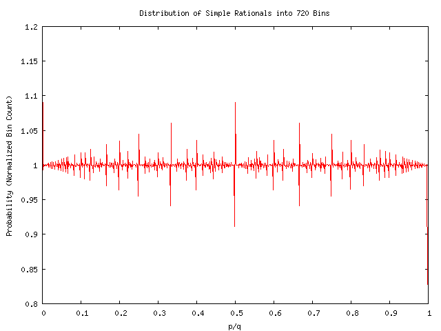
The figure ![]() shows this enumeration, up to a denominator
of K=4000, carved up into N=720 bins, and normalized to unit density.
That is, if
shows this enumeration, up to a denominator
of K=4000, carved up into N=720 bins, and normalized to unit density.
That is, if
![]() , then we assign the fraction
, then we assign the fraction
![]() to the
to the ![]() 'th bin, and so the graph is a histogram. We might
expect this graph to have a huge peak at the bin n=360: after all,
this bin will hold 1/2 and 2/4 and 3/6 and in general should have
a big surfiet coming from the degeneracy at 1/2. One mght expect peaks
at 1/3, and 1/4 and etc, but smaller.
'th bin, and so the graph is a histogram. We might
expect this graph to have a huge peak at the bin n=360: after all,
this bin will hold 1/2 and 2/4 and 3/6 and in general should have
a big surfiet coming from the degeneracy at 1/2. One mght expect peaks
at 1/3, and 1/4 and etc, but smaller.
The above is a density graph of the rationals that occur in the simple enumeration, binned into 720 bins, up to a denominator of N=4000. The normalization of the bin count is such that the expected value for each bin is 1.0, as explained in the text. |
Indeed, there is a big upwards spike at 1/2. But there seems to be a big downwards spike just below, at bin 359, seemingly of equal and opposite size. This is the first surprise. Why is there a deficit at bin 359? We also have blips at 1/3, 1/4, 1/5, 1/6, but not at 1/7: something we can hand-wave away by noting that 720 is 6 factorial. (When one attempts 7!=5040 bins, one finds the peak at 1/7 is there, but the one at 1/11 seems to be missing; clearly having the number of bins being divisible by 7 is important.). The other surprising aspect of this picture is the obvious fractal self-similarity of this histogram. The interval between 1/3 and 1/2 seems to reprise the whole. The tallest blip in the middle of this subinterval occurs at 2/5, which is the Farey mediant of 1/2 and 1/3. Why are we getting something that looks like a fractal, when we are just counting rationals? More tanalizingly, why does the fractal involve Farey Fractions?
We suspect that something peculiar happens because the over-counting at 1/2, 2/4'ths etc. falls on exactly the boundary between bins 360 and 359. In fact, any fraction with a denominator that is a multiple of 2,3,4,5, or 6 will have this problem; fractions that have a multiple of 7 in the denominator don't seem to have this problem, perhaps because they are not on a bin boundary. We can validate this idea by binning into 719 bins, noting that 719 is prime. Thus, for the most part, almost all fractions will clearly be in the ``middle'' of a bin. We expect a flatter graph; the up-down blips should cancel. But it shouldn't be too flat: we still expect a lot of overcounting at 1/2. See below:
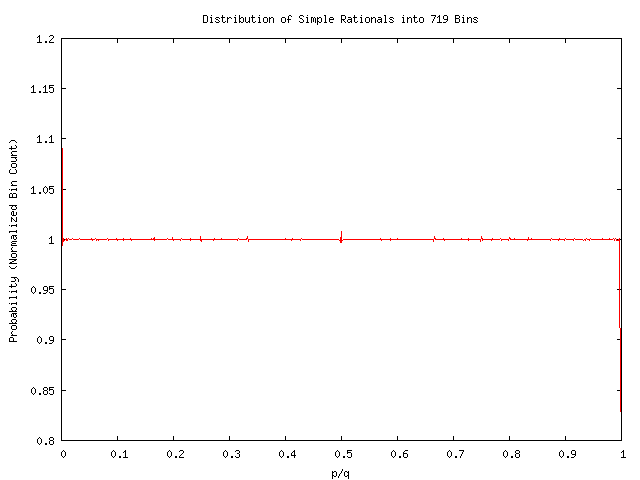
Wow, thats flat! How can this graph possibly be so flat? We should be massively overcounting at 1/2, there should be a big peak there. Maybe its drowned out by the blips at 0 and 1: we are, after all histograming over 8 million fractions, and we expect statistical variations to go as one over the sqaure-root of the sample size. So lets graph the same data, but rescale more appropriately. This is shown below:
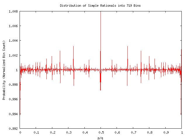
Hmm. Curious. There is indeed a peak at 1/2. But there are also deficits symmetrically arranged at either side. This is still confusing. We might have expected peaks, but no deficits, with the baseline pushed down, to say, 0.999, with all peaks going above, so that the total bin count would still average out to 1.0. But the baseline is at 1.0, and not at 0.999, and so this defies simple intuition. Notice also that the fractal nature is still evident. There are also peaks at 1/3, 1/4, 1/5 and 1/6. But not at 1/7'th. Previously, we explained away the lack of a peak at 1/7'th by arguing about the prime factors of 720; this time, 719 has no prime factors other than itself; thus, this naive argument fails. What do we replace this argument with?
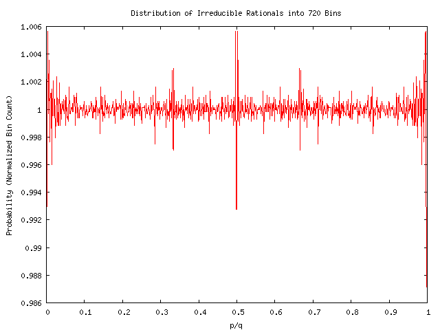
Well, at any rate, lets compare this to the distribution we ``should have been using all along'', where we eliminate all fractions that are reducible. That is, we should count each rational only once. This mkes a lot more sense, if we are to talk of teh distribution of rationals on the real number line. This is graphed below, again, binned into 719 bins, for all irreducible rationals with denominator less than or equal to 4000:
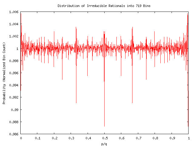
Wow! We no longer have a peak at 1/2. In fact, it sure gives the distinct impression that we are undercounting at 1/2! Holy Banach-Tarski, Batman! What does it mean? Note also the graph is considerably noiser. Compare the scales on the left for a relative measure of the noise. Part, but not all, of the noise is due to the smaller sample size: we are counting fewer fractions: 4863602 are irreducible out of the simple list of 8002000. However, matching the sample sizes does not seem to significantly reduce the small-amplitude noise: qualitatively speaking, the binning of irreducible fractions seems much noisier.
Let us pause for a moment to notice that this noise is not due to
some numerical aberation due to the use of floating-point numbers,
IEEE or otherwise. The above bincounts are performed using entirely
integer math. That is, for every pair of integers ![]()
![]() , we computed
the integer bin number
, we computed
the integer bin number ![]() and the integer remainder
and the integer remainder ![]() such that
such that ![]() holds as in integer equation, where
holds as in integer equation, where ![]() was
the number of bins. This equation does not have 'rounding error' or
'numerical imprecision'.
was
the number of bins. This equation does not have 'rounding error' or
'numerical imprecision'.
Curiously, binning into a non-prime number of bins does seem to reduce the (small-amplitude) noise. Equally curiously, it also seems to erase the prominent features that were occuring ath the Farey Fractions. This is exactly the opposite of the previous experience, where it was bining to a prime that seemed to 'erase' the features. Below is the binning into 720 bins.
Following the usual laws of statistics and averages, one expects that increasing the sample size reduces the noise. This is true in an absolute sense, but not a relative sense. The graph below shows 720 bins holding all irreducible rationals with denominators less than 16000. The absolute amplitude has been reduced by over a factor of ten compared to the previous graphs; this is not a surprise. We are counting 77809948 irreducible rationals, as opposed to 4863602 before: our sample size is nearly 16 times larger. What is perhaps surprising is that there is relatively far more power in the higher frequencies. There are also still-visible noise peaks near 1/2, 1/3, and 2/3'rds, as well as at 0 and 1.
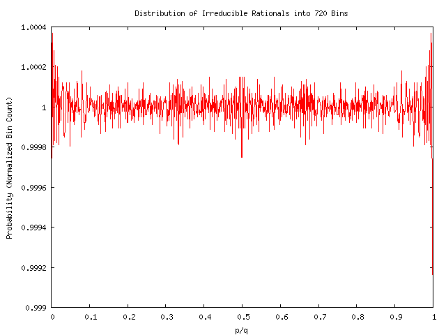
Let reiterate that the noise in this figue is not due to floating-point errors or numerical imprecision. Its really there, deeply embedded in the rationals. As we count more and more rationals, and bin them into a fixed number of bins, then we will expect that the mean deviation about the norm of 1.0 to shrink and shrink, as some power law. It is in this sense that we can say that the rationals are uniformly distributed on the real-number line: greater sample sizes seemingly leads to more uniform distributions, albeit with strangely behaved variances. But even this statement is less than conclusive, because it hides a terrible scale invarience. We have one more nasty histogram to demonstrate.
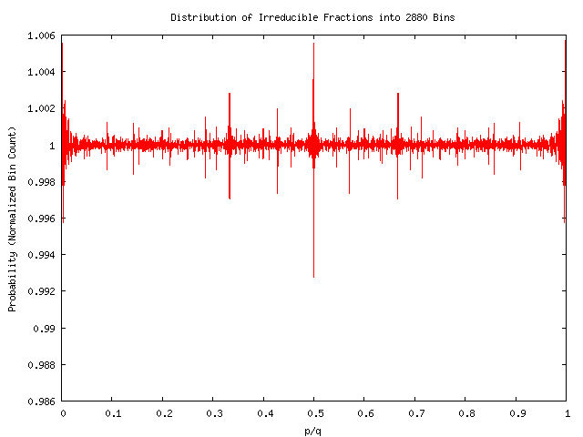
This one shows irreducible fractions with denominators less than 16000, which, as we've mentioned, represents a sample size almost 16 times larger than the first sets of graphs. We bin these into four times as many bins: 2880=4x720. Compare the normalized scale on the vertical axis to the corresponding picture for the smaller sample size and smaller number of bins. The vertical scales are identical, and the sizes of the peaks are identical. Each bin, on average, holds four times as many rationals (16 times as many rationals, 4 times as many bins). We've increased our sample size, but the features are not 'washing out': they are staying constant in size, and are becoming more distinct and well-defined.
In light of the fact that the above graphs have some surprising features, we take a moment to try to be precise about what we mean when we say ``histogram'' and ``normalize''.
Lets go back to the first figure. The total number of rationals in
the histogram is
![]() , a little over
eight million: a decent sample size. Each bin will have some count
, a little over
eight million: a decent sample size. Each bin will have some count
![]() of these rationals. We want to talk in statistical terms,
so we normalize the bin count as
of these rationals. We want to talk in statistical terms,
so we normalize the bin count as
![]() , so that
the average value or expected value of
, so that
the average value or expected value of ![]() is 1.0. That is, we
have, by definition,
is 1.0. That is, we
have, by definition,
The act of bining a rational ![]() requires a division; that is,
in order to determine if
requires a division; that is,
in order to determine if
![]() , a division is unavoidable.
However, we can avoid numerical imprecision by sticking to integer
division; using floating point here potentially casts a cloud over
any results. With integer division, we are looking for
, a division is unavoidable.
However, we can avoid numerical imprecision by sticking to integer
division; using floating point here potentially casts a cloud over
any results. With integer division, we are looking for ![]() such that
such that
![]() ; performing this computation requires no rounding
or truncation. The largest such integers we are likely to encounter
in the previous sections are
; performing this computation requires no rounding
or truncation. The largest such integers we are likely to encounter
in the previous sections are
![]() , for which
ordinary 32-bit math is perfectly adequate; there is no danger of
overflow. If one wanted to go deeper, one could use arbitrary precision
libraries; for example, the Gnu Bignum Library, GMP, is freely available.
But the point here is that to see these effects, one does not need
to work with numbers so large that arbitrary precision math libraries
would be required.
, for which
ordinary 32-bit math is perfectly adequate; there is no danger of
overflow. If one wanted to go deeper, one could use arbitrary precision
libraries; for example, the Gnu Bignum Library, GMP, is freely available.
But the point here is that to see these effects, one does not need
to work with numbers so large that arbitrary precision math libraries
would be required.
So what is it about the rational numbers that makes them behave like this? Lets review some basic properties.
We can envision an arbitrary fraction ![]() made out of the integers
made out of the integers
![]() and
and ![]() as corresponding to a point
as corresponding to a point ![]() on a square lattice.
This lattice is generated by the vectors
on a square lattice.
This lattice is generated by the vectors ![]() and
and ![]() :
these are the vectors that point along the x and y axes. Every point
on the lattice can be represented by the vector
:
these are the vectors that point along the x and y axes. Every point
on the lattice can be represented by the vector
![]() for some integers
for some integers ![]() and
and ![]() . This grid is a useful way to think
about rationals: by looking out onto this grid, we can ``see''
all of the rationals, all at once.
. This grid is a useful way to think
about rationals: by looking out onto this grid, we can ``see''
all of the rationals, all at once.
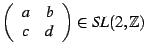
 . The set of all matrices with determinant equal to
 then
then
Next, we've learned that the symmetries of a square grid are hyperbolic.
Of course, everyone knows that square grids have a translational symmetry;
we didn't even mention that. Square grids don't have a rotational
symmetry, except for rotations by exactly 90 degrees. But only a few
seem to know about the ``special relativity'' of a square lattice.
Just like ``real'' special relativity, there is a strange squashing
and shrinking of lengths while a ``cell'' or ``fundamental
region'' is squashed. Worse, this group
![]() , known
as the modular group, is implicated in a wide variety of hyperbolic
goings-on. It is a symmetry group of surfaces with constant negative
curvature (the Poincare upper half-plane). All sorts of interesting
chaotic phenomena happen on hyprbolic surfaces: geodesics diverge
from each other, and are thus said to have positive Lyapunov exponent,
and the like. The Riemann zeta function, and its chaotic layout of
zeros (never mind the chaotic layout of the prime numbers) are closely
related. In general, whenever one sees something hyperbolic, one sees
chaos. And here we are, staring at rational numbers and seeing something
hyperbolic.
, known
as the modular group, is implicated in a wide variety of hyperbolic
goings-on. It is a symmetry group of surfaces with constant negative
curvature (the Poincare upper half-plane). All sorts of interesting
chaotic phenomena happen on hyprbolic surfaces: geodesics diverge
from each other, and are thus said to have positive Lyapunov exponent,
and the like. The Riemann zeta function, and its chaotic layout of
zeros (never mind the chaotic layout of the prime numbers) are closely
related. In general, whenever one sees something hyperbolic, one sees
chaos. And here we are, staring at rational numbers and seeing something
hyperbolic.
It is also worth noting that the square grid, while being a cross-product
![]() of integers, is not a free product.
By this we mean that there are multiple paths from the origin to any
given point on the grid: thus, to get to
of integers, is not a free product.
By this we mean that there are multiple paths from the origin to any
given point on the grid: thus, to get to ![]() , we can go right
first, and then up, or up first, and then right. Thus the grid is
actually a quotient space of a free group. (XXX need to expand on
this free vs. quotient thing).
, we can go right
first, and then up, or up first, and then right. Thus the grid is
actually a quotient space of a free group. (XXX need to expand on
this free vs. quotient thing).
To conclude, we've learned the following: the set of rationals ![]() consists entirely of the set of points on the grid that are visible
from the origin. The entire set of rationals can be generated from
just a pair of rationals
consists entirely of the set of points on the grid that are visible
from the origin. The entire set of rationals can be generated from
just a pair of rationals ![]() and
and ![]() , as long as
, as long as ![]() .
By ``generated'' we mean that every rational number can be written
in the form
.
By ``generated'' we mean that every rational number can be written
in the form
One oddity that we should notice is the superficial resemblance to
Farey addition: given two rational numbers ![]() and
and ![]() , we add
them not as normal numbers, but instead combining the numerator and
denominator. As we will see, Farey fractions and the modular group
are intimately intertwined.
, we add
them not as normal numbers, but instead combining the numerator and
denominator. As we will see, Farey fractions and the modular group
are intimately intertwined.
The symmetries of the histograms are given by
![]() ,
a fact that we develop in later chapters. (XXX see the other pages
on this website for now). Just to provide a taste of what is to come,
here's a picture of the orbit of a vector under the action of the
group elements of the dyadic representation of the modular group:
,
a fact that we develop in later chapters. (XXX see the other pages
on this website for now). Just to provide a taste of what is to come,
here's a picture of the orbit of a vector under the action of the
group elements of the dyadic representation of the modular group:
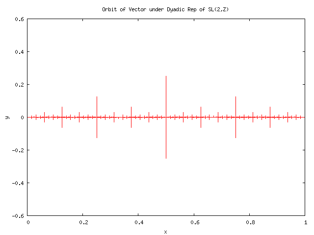
That is, we consider how the vector ![]() transforms under
the group elements generated by
transforms under
the group elements generated by
In this representation, the only naturally occuring numbers are of
the form ![]() , and so the main sequence of the peaks are rooted
at 1/2, 1/4, 1/8 etc. To get to the peaks occuring at the Farey numbers,
we need to work through the Minkowksi Question mark function, which
provides the isomorphism between the Farey Numbers and the Dyadics.
(This is done in the next chapter). (XXXX we really need to re-write
this section so it doesn't have to allude to the 'other stuff').
, and so the main sequence of the peaks are rooted
at 1/2, 1/4, 1/8 etc. To get to the peaks occuring at the Farey numbers,
we need to work through the Minkowksi Question mark function, which
provides the isomorphism between the Farey Numbers and the Dyadics.
(This is done in the next chapter). (XXXX we really need to re-write
this section so it doesn't have to allude to the 'other stuff').
As to the origin of the (white) noise, a better perspective can be gotten on the chapter on continued fraction gaps.
Write me. Introduce the next chapter.
This is kind-of a to-do list.
It sure would be nice to develop a generalized theory that can work with these peculiar results, and in particular, giving insight into what's happening near 1/2 and giving a quantitative description of the spectra near 1/3 and 2/3, etc. We want to graph the mean-square distribution as a function of sample size. We want to perform a frequency analysis (fourrier transform) and get the power spectrum.
When we deal with a finite number of bins, we cannot, of course, get the full symmetry of the modular group. For a finite number of bins, we expect to see the action of only some finite subgroup (or subset) of the modular group. What is that subgroup (subset)? What are its properties?
We also have a deeper question: we will also need to explain why the
modular group shows up when one is counting rationals; we will do
this in the next chapter, where we discuss the alternate representations
of the reals. Its almost impossible to avoid.