Additional explorations of the interior can be found in the M-Set Derivations Room and the Spectral Analysis Room.
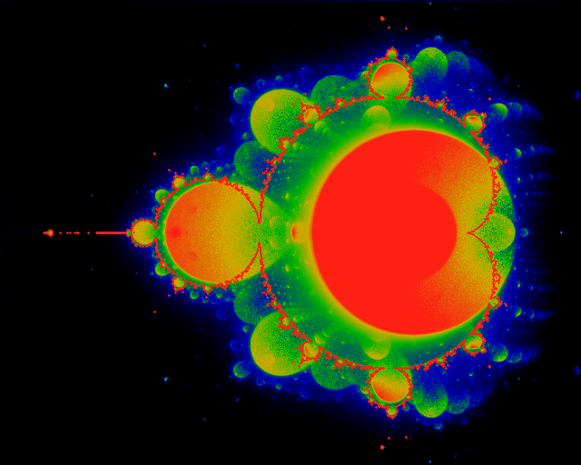
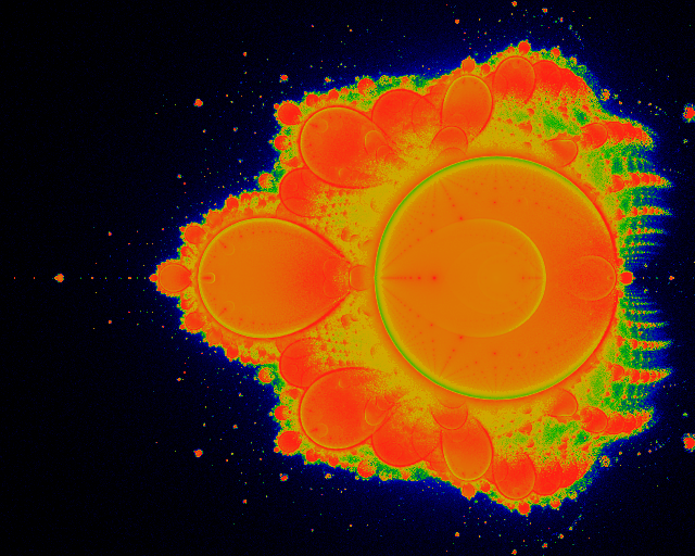
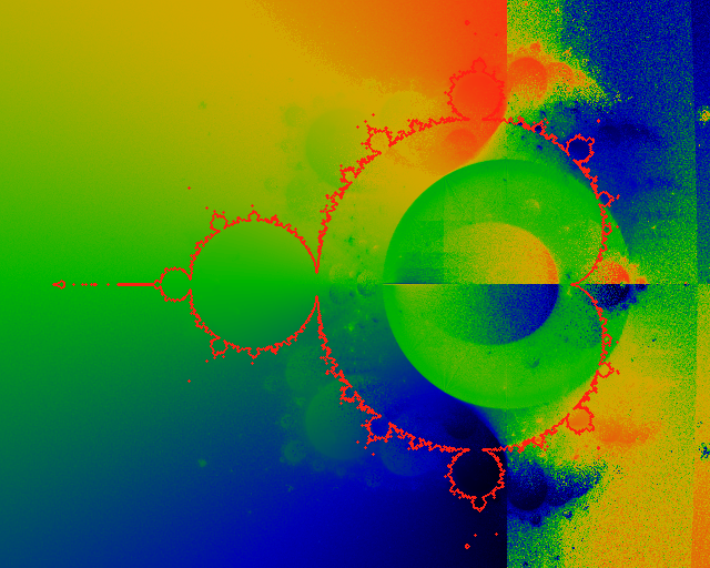
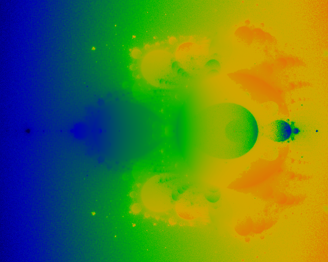
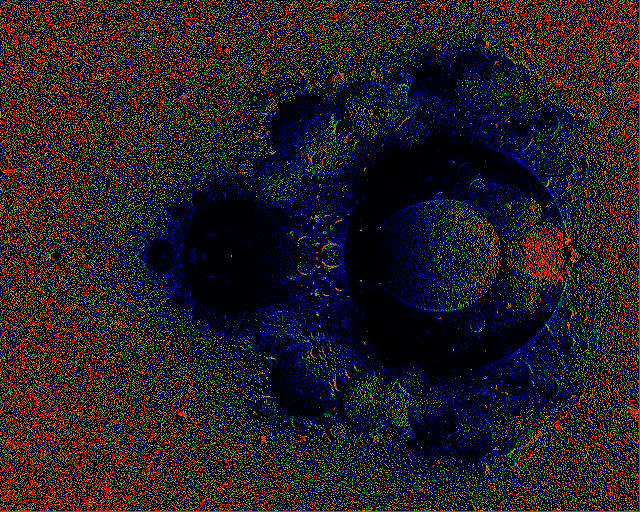
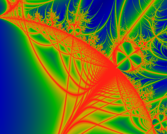
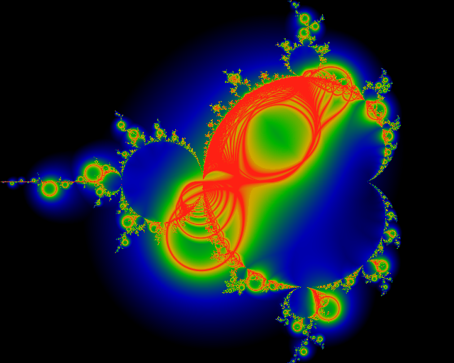
Hausdorf measure of Mandelbrot Interior. This picture is created by
dividing up the complex plane into pixels, and counting how many times
each pixel is visited as the iterator is iterated. Red pixels are
visited often; yellow, green, blue and black, respectively, less so.
The red outline shows boundary of set, as usually seen.
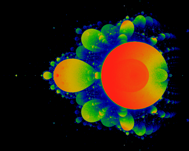
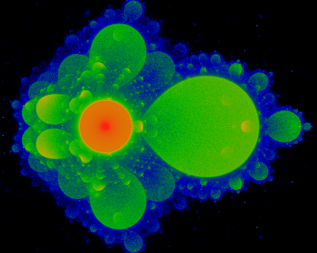
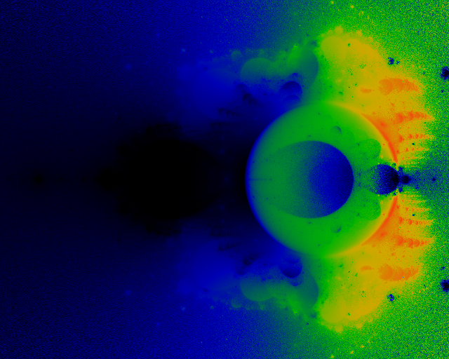
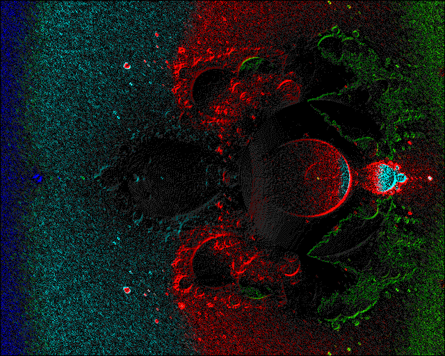
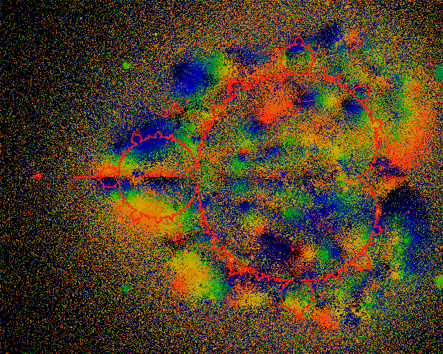
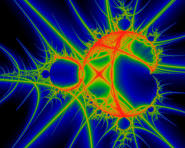
 Lyapunov Exponent of iterates. Red indicates a large positive
(divergent) exponent, moving through yellow, green and blue to black,
which indicates a small or negative (attractive) exponent.
Lyapunov Exponent of iterates. Red indicates a large positive
(divergent) exponent, moving through yellow, green and blue to black,
which indicates a small or negative (attractive) exponent.
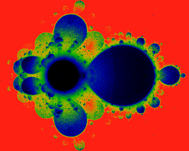
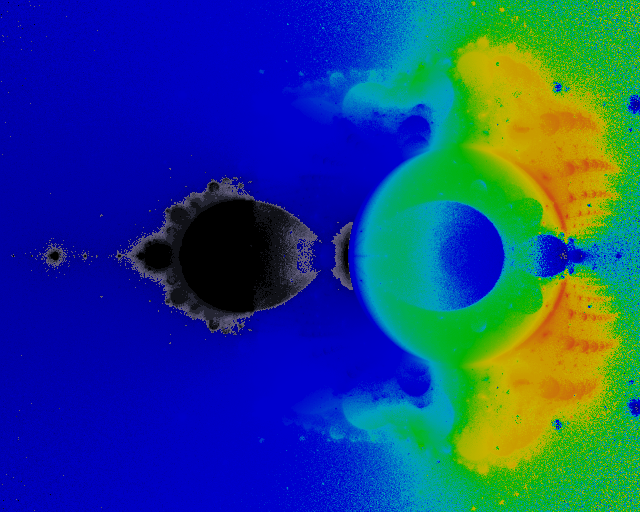
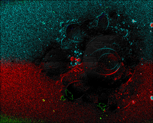
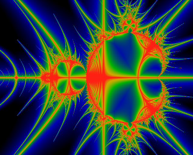
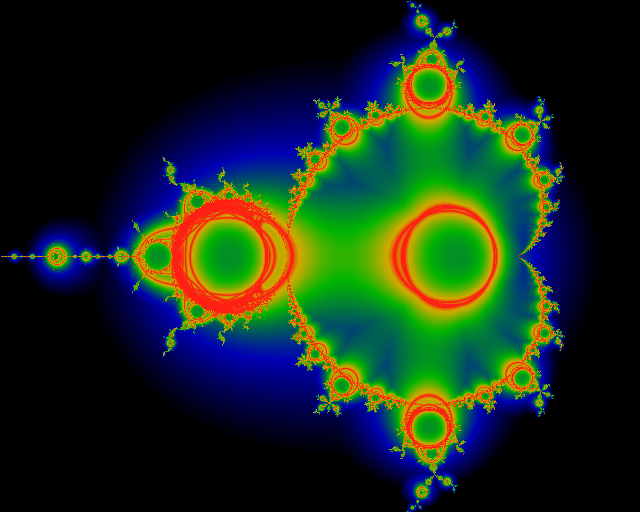
 Lyapunov Exponent of iterates, this time showing the attractive strength.
Red shows regions of strong attraction. Note that it appears that
some of the attractors lie outside the Mandelbrot set. Note that these
attractors seem to correspond to zeros of iterates of various orders.
(See below).
Lyapunov Exponent of iterates, this time showing the attractive strength.
Red shows regions of strong attraction. Note that it appears that
some of the attractors lie outside the Mandelbrot set. Note that these
attractors seem to correspond to zeros of iterates of various orders.
(See below).
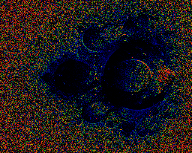
 Hausdorf measure at very high iterations ... allowed to iterate a far,
far longer time. Note that some of the "fuzz" goes away.
Hausdorf measure at very high iterations ... allowed to iterate a far,
far longer time. Note that some of the "fuzz" goes away.
 Average age. That is, cycle count at which pixel was hit were accumulated,
and then normalized by the measure at that pixel.
Average age. That is, cycle count at which pixel was hit were accumulated,
and then normalized by the measure at that pixel.
 Mean square deviation in the "age". Note how different details are
highlighted.
Mean square deviation in the "age". Note how different details are
highlighted.
 Third moment of the "age". Further details not appearent in the measure or
the Lyapunpov exponents become visible.
Third moment of the "age". Further details not appearent in the measure or
the Lyapunpov exponents become visible.
 Fourth moment of the "age". Further details not appearent in the measure or
the Lyapunpov exponents become visible.
Fourth moment of the "age". Further details not appearent in the measure or
the Lyapunpov exponents become visible.
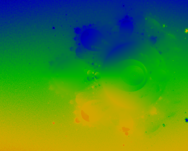
 Hausdorff measure, revisited. The iterated equation is still
z = z*z +C, except that in this picture, we show the visited areas
relative to C (i.e. we subtract C from z prior to plotting). Note that
the circle (red dot) is centered about the origin. The origin is offset
to show the large lobe to the right.
Hausdorff measure, revisited. The iterated equation is still
z = z*z +C, except that in this picture, we show the visited areas
relative to C (i.e. we subtract C from z prior to plotting). Note that
the circle (red dot) is centered about the origin. The origin is offset
to show the large lobe to the right.
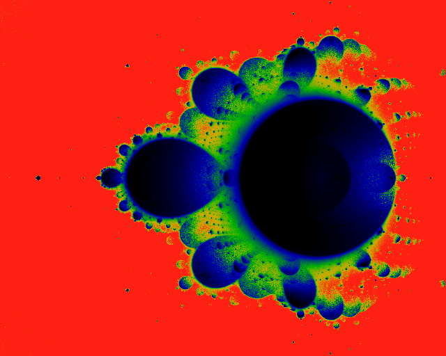
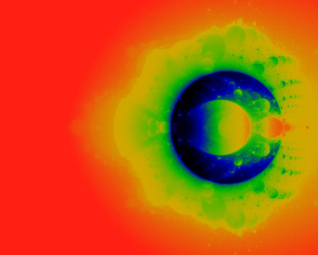
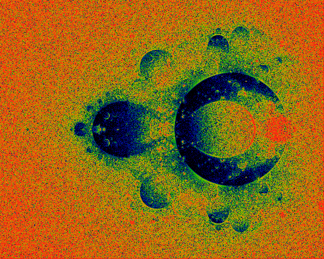
 Lyapunov exponenet. All non-black regions are replusive, with red
representing the most strong repulsive regions.
Lyapunov exponenet. All non-black regions are replusive, with red
representing the most strong repulsive regions.
 Square distance between iterations; i.e (x-xlast)^2 + (y-ylast)^2
acumulated and normalized.
Square distance between iterations; i.e (x-xlast)^2 + (y-ylast)^2
acumulated and normalized.
 Gaussian edge filter applied to above.
 Average orientation (angle) of jump, where a "jump" is the vector from
the last to the current location. That is,
phi = arctan ((y-ylast)/(x-xlast)) accumualted and normalized.
Average orientation (angle) of jump, where a "jump" is the vector from
the last to the current location. That is,
phi = arctan ((y-ylast)/(x-xlast)) accumualted and normalized.
 Cosine of angle between current jump and last jump. The colormap used
shows black = 0.0 (angle=90), red=1.0 (angle = 0).
This is a very nice spirit-catcher, on it's side.
Cosine of angle between current jump and last jump. The colormap used
shows black = 0.0 (angle=90), red=1.0 (angle = 0).
This is a very nice spirit-catcher, on it's side.
 A different colormap brings out different detail.
 Average X origin. The is, each pixel shows the average value of the
real part of C where z = z2+C.
Average X origin. The is, each pixel shows the average value of the
real part of C where z = z2+C.
 Average Y origin. The is, each pixel shows the average value of the
imaginary part of C where z = z2+C.
Average Y origin. The is, each pixel shows the average value of the
imaginary part of C where z = z2+C.
 Edge detection applied to average X origin.
 Edge detection applied to average Y origin.
 Curl (dxY - dyX) of the average origin (X, Y). Curiously, the
Divergence (dxX + dyY) looks qualitatively similar.
Curl (dxY - dyX) of the average origin (X, Y). Curiously, the
Divergence (dxX + dyY) looks qualitatively similar.
 Curl, as above, but with slightly different colormap.
 Divergence. Note qualitative similarities, and subtle differences (which
help reveal some of the minute artifacts in the other images).
Divergence. Note qualitative similarities, and subtle differences (which
help reveal some of the minute artifacts in the other images).
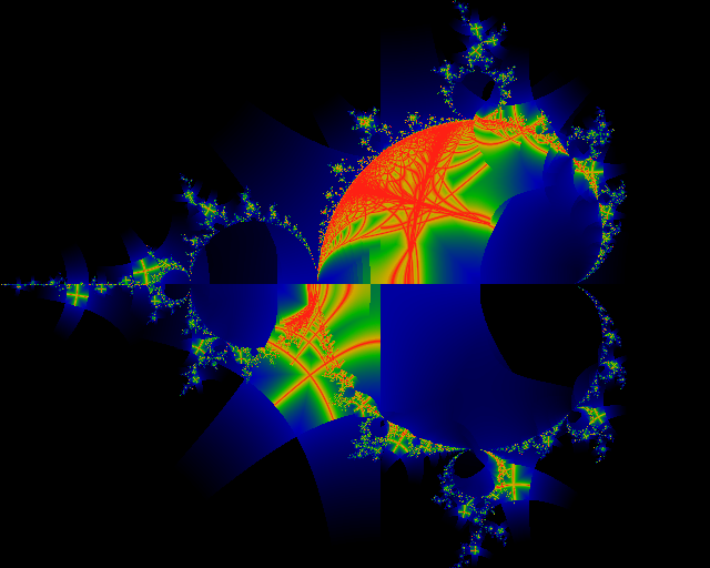
 Splat. Just a splat. Note the spiral structure, bottom center. How to
clean this up ??
Splat. Just a splat. Note the spiral structure, bottom center. How to
clean this up ??
 Origins -- X. That is, each point is colored with the real part of C where
z = z2 + C. Unlike the average origins image above, this is done with
a "last point wins" coloring.
Origins -- X. That is, each point is colored with the real part of C where
z = z2 + C. Unlike the average origins image above, this is done with
a "last point wins" coloring.
 Fine origins -- X. As above, but different colormap.
 Origins -- Y.
 Fine origins -- Y.
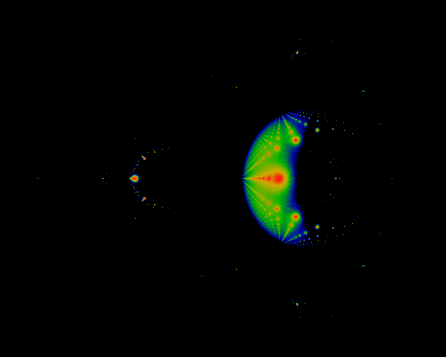
 Pickover's Stalks. Cliff Pickover hit on the novel concept of looking
to see how closely the orbits of interior points come to the x and y
axes. In these pictures, the closer that the point approaches, the
higher up the color scale, with red denoting the closest approach. The
logarithm of the distance is taken to accentuate the details.
Pickover's Stalks. Cliff Pickover hit on the novel concept of looking
to see how closely the orbits of interior points come to the x and y
axes. In these pictures, the closer that the point approaches, the
higher up the color scale, with red denoting the closest approach. The
logarithm of the distance is taken to accentuate the details.
 A closeup of the upper left area.
 How close do iterates come to the horizontal and vertical axes centered
at (-0.25, 0.25) ?
How close do iterates come to the horizontal and vertical axes centered
at (-0.25, 0.25) ?
 How closely do iterates approach the cross, defined as (0==x,
-0.2<y<0.2) + (-0.2<x<0.2, 0==y) ?
How closely do iterates approach the cross, defined as (0==x,
-0.2<y<0.2) + (-0.2<x<0.2, 0==y) ?
 How closely do iterates approach the cross centered at (-0.3, 0.2) ?
 Note that the previous images showed that some points inside every bud
iterated quite close to the origin. Naively, it might seem that some
point inside every bud iterates closely to some point inside the main
cardiod. For example:
How closely do iterates approach the circle, centered at the origin,
of radius 0.2?
Note that the previous images showed that some points inside every bud
iterated quite close to the origin. Naively, it might seem that some
point inside every bud iterates closely to some point inside the main
cardiod. For example:
How closely do iterates approach the circle, centered at the origin,
of radius 0.2?
 How closely do iterates approach the circle, centered at (-0.3, 0.2),
of radius 0.2?
How closely do iterates approach the circle, centered at (-0.3, 0.2),
of radius 0.2?
The first image was created in 1988, as were variations on some of the others. All electronic copies were lost, with only polaroids and proof sheets surviving. New electronic copies were recreated in 1996 for this web exhibit.
Copyright (c) 1988, 1990, 1996, 1997 Linas Vepstas

Mandelbrot Interior
by Linas Vepstas is licensed under a
Creative Commons
Attribution-ShareAlike 4.0 International License.